4.4. Parameter sensitivity analysis

Important

This tutorial is only compatible with ParAMS 2023.1 or later.

This example builds on ReaxFF (basic): H₂O bond scan. That example focuses on the optimization, this one focuses on the parameter sensitivity analysis.

When reparameterizing ReaxFF it is difficult to know which parameters to optimize.

• Too few parameters might make it difficult to find a good fit.

• Too many parameters will make the optimization harder, slower, and increase the risk of overfitting.

In this tutorial we will show you how to identify the most sensitive parameters which can guide your parameter selection.

The relevant files for this tutorial can be found in $AMSHOME/scripting/scm/params/examples/ReaxFF_water.

See also

How to run a sensitivity job from Python.

4.4.1. How sensitivity is calculated

Sensitivity is calculated using the Hilbert-Schmidt Independence Criteria (HSIC), a robust and popular kernel-based dependence measure.

• The HSIC equals zero if and only if variables are independent

• Larger values imply higher dependency between variables

We will test the dependency of the loss function on each of the parameters we might consider optimizing.

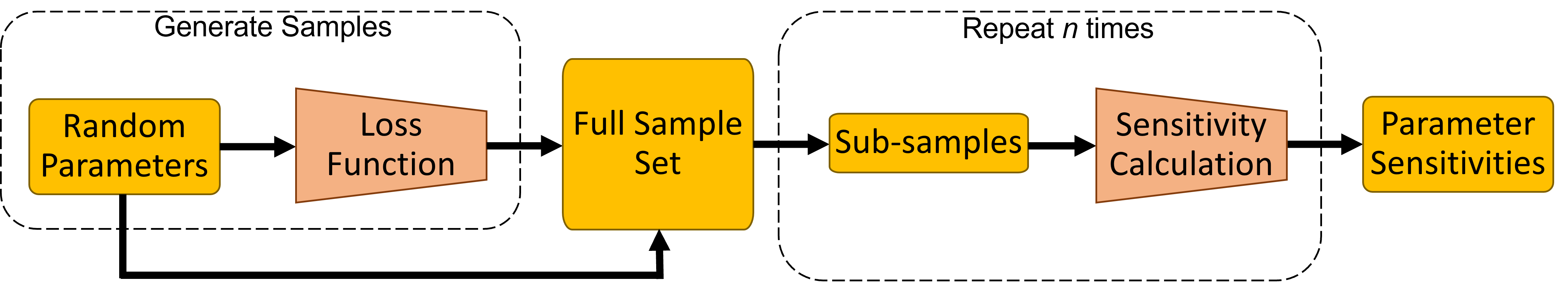
Fig. 4.6 Simplified sensitivity workflow schematic

The sensitivity calculation is performed as follows:

1. Select all the parameters you would like to investigate

2. Draw uniform random samples of parameters values

3. Calculate loss values for each of the parameter sets

4. For each parameter calculate the HSIC metric using the parameter values and loss function values

5. Calculate sensitivity values based on the HSIC metric

Sensitivity values have two properties which make them very easy to interpret:

• all sensitivity values sum to one;

• a sensitivity value ranges from 0 (insensitive) to 1 (sensitive);

4.4.2. Setting up a sensitivity calculation

First load the example files:

Open the ParAMS GUI: SCM → ParAMS

File → Open

Select sensitivity.in.

This will load the sensitivity calculation inputs and the YAML files.

Warning

Do not select another file when opening since this will default to the input file called params.in which is the setup for the optimization version of this tutorial.

4.4.2.1. Selecting parameters

Next we consider the parameters we would like to investigate.

On the Parameters panel select the Active dropdown

Unselect Show Non-Active

This shows that all 12 parameters related to an H.O bond are active.

If we consider the parameter descriptions we see that 6 of them are associated with π-bonds which are not present in the training set, so they should have no influence on the optimization.

Instead of deactivating these parameters, we will leave these parameters active as a test of the sensitivity method.

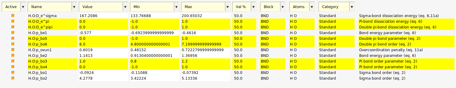
Fig. 4.7 12 active parameters with parameters related to π-bonds selected.

4.4.2.2. Input options

We will now configure the sensitivity calculation.

Click to open the input panel

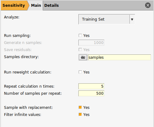
4.4.2.2.1. Set To Analyze

The Analyze option allows you to select if you would like to test the sensitivity of the training set or the validation set.

Investigating both can be very helpful in understanding why the two perform differently.

In this tutorial, we have no validation set and thus test only the training set.

4.4.2.2.2. Loading/Generating Samples

The second set of options relate to producing or loading the samples of the loss function. If you have produced samples before, you can use them again for a different sensitivity calculation to save time because sampling takes longer than the sensitivity calculation.

In this tutorial you can choose to either

• Load samples from the sample directory (to get through the tutorial quicker), or

• Generate the samples yourself (if no samples had been generated previously, this would be a necessary step)

To load samplesTo generate samples

Deactivate Run Sampling

This enables the Samples Directory option

Click and select the samples directory in the example directory

The associated input keys for loading samples:

RunSampling No
SamplesDirectory path/to/samples

In general the Samples Directory must have the following structure:

samples_directory
├── training_set_results (or validation_set_results)
│   ├── running_active_parameters.txt
│   └── running_loss.txt
└── glompo_log.h5

• Only glompo_log.h5 or the running_*.txt files are needed.

• If glompo_log.h5 is present, it will take precedence.

• glompo_log.h5 is produced by saving residuals (see the To generate samples tab).

Tip

Sampling will produce a directory called sampling_results within the results directory. To load these samples point Samples Directory to: results/sampling_results/optimization.

4.4.2.2.3. Samples used in calculation

Our pool of samples contains 2000 samples. To take full advantage of these we can:

• Use all 2000 samples in a single calculation; or

• Take a subset of the samples, run a smaller calculation, and repeat this for different subsets.

It is always recommended to repeat the sensitivity calculation. The spread of results will tell you if you have enough samples. It is usually cheaper to repeat a calculation with subsets of samples than run it is to run it using all samples once.

We will repeat the calculation five times using subsets of 500 samples each time.

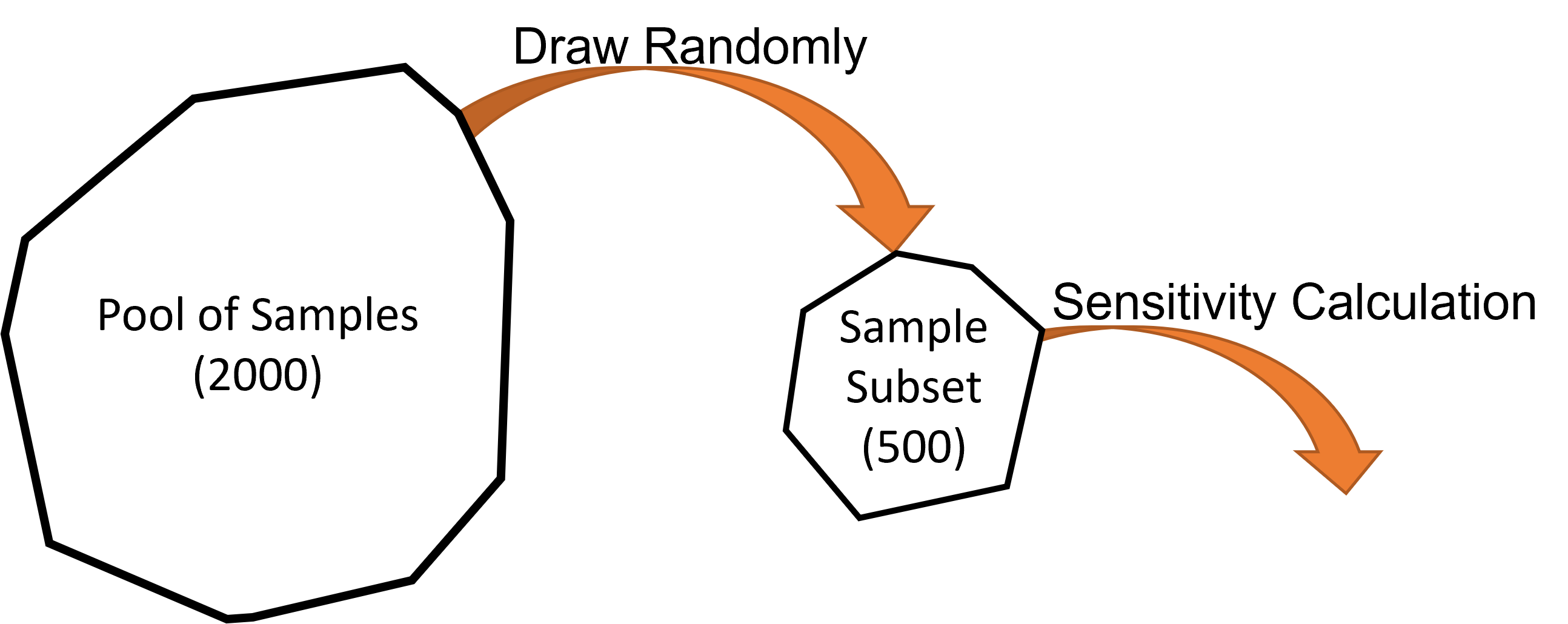
Fig. 4.8 The sensitivity calculation is run on a subset of of the pool of samples.

Set Repeat calculation n times to 5

Set Number of samples per repeat to 500

A new subset is drawn from the full pool for every calculation repeat.

If Sample with replacement is Yes then the subset can contain repeated samples from the full pool of samples. Otherwise, a sample can only appear once in a subset.

If Filter infinite values is Yes then any samples with an infinite loss function value will not be included in the full pool of samples.

Tip

If Run Reweight Calculation is Yes, then the sensitivity calculation is extended to provide suggested training set weights which should provide a better balance of sensitivities for the parameter set. This training set only has one item so we will not run the reweight calculation.

Data sets which are imbalanced can be harder to optimize. A reweight calculation

• suggests new training set weights,

• reveals dependencies within the training set,

• can help to guide training set design.

Unfortunately, a reweight calculation is much more computationally demanding than a regular sensitivity calculation.

4.4.2.2.4. Choosing Kernels

The key sensitivity calculation inputs are kernels. We need two kernels:

• a kernel to quantify the dis/similarity between parameter values;

• a kernel to classify the loss function values.

On the input panel, Details → Kernels

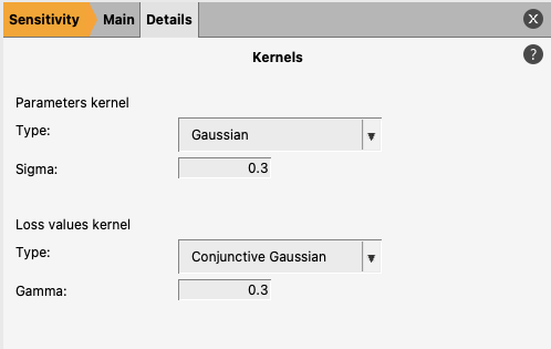
The default kernels should be sufficient in most scenarios.

The default parameter values kernel applies a Gaussian kernel to the parameter values. This measures the distance between parameter values and applies no underlying assumption on the shape of the distribution of parameter values.

The default loss values kernel is a conjunctive-Gaussian type kernel which places the bulk of its distribution on the lowest loss values. This helps identify small local sensitivities near the minima we are interested in which might otherwise be drowned out by large global sensitivities.

4.4.3. Sensitivity results

Save and run the calculation:

File → Save

Save the calculation as watersensi.params

File → Run

The calculation should take a couple of seconds. You can see progress and get an estimated completion time from the progress bar printed in the logfile.

4.4.3.1. Graphical results

Once complete the GUI will show 2 summary plots:

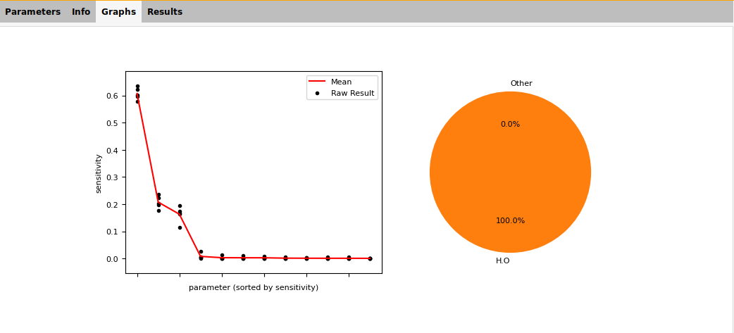
Fig. 4.9 Example sensitivity result summary provided by the GUI

The scatter plot shows:

• the sensitivity result for each parameter for each repeat (black dots);

• the mean sensitivity for each parameter (red line).

This does not identify particular parameters, but one can see:

• the number of parameters which dominate the sensitivity;

• if there is a large spread between repeats (means more samples are needed).

In this example:

• we detect significant sensitivity for only three parameters;

• the spread between repeats is robust and does not influence the ordering of parameters.

The pie chart shows the allocation of sensitivity to different groups. For ReaxFF, the groups are atoms and blocks combinations. Here we only analysed parameters in the H.O bond block, so all of the sensitivity is in that group.

4.4.3.2. Sensitivity values

Close the panel if it is open

Switch to the Parameters panel

Click the Active column header and deselect Show Non-Active

Click the Sensitivity column header and click Sort Decreasing

Tip

You might have to resize your window to see the Sensitivity and Description columns

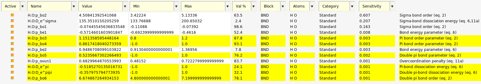
Fig. 4.10 12 active parameters and their calculated sensitivities with parameters related to π-bonds selected.

Each active parameter has been given the average sensitivity value from the repeats (seen as the red line on the plot).

In our results we see:

• negligible sensitivity was detected for the π-bond related parameters;

• H.O:p_be1, H.O:p_be2 and H.O:p_ovun1 are also found to be insensitive;

• Most of the sensitivity is divided between three σ-bond related parameters.

4.4.3.3. Results files

The results for a sensitivity calculation have the following structure:

jobname.results
├── sampling_results (if samples generated)
│   ├── settings_and_initial_data
│   └── optimization (directory to chose when loading samples)
├── settings_and_initial_data
│   └── data_sets
└── sensitivity
    ├── calculation_result.npz
    ├── parameter_interface_with_sensitivities.yaml
    ├── sensitivity_per_parameter.png
    ├── sensitivity_summary.png
    └── sensitivity_summary.txt

• calculation_result.npz contains the calculation results and the inputs which can be loaded in Python:

  from scm.glompo.analysis.hsic import HSICResult
  
  if __name__ == '__main__':
      result = HSICResult.load('path/to/calculation_result.npz')
  

  For more details see the API documentation

• parameter_interface_with_sensitivities.yaml is the normal parameter interface YAML file with a sensitivity metadata key for all the parameters. The key is blank if the parameter was not ‘active’ for the calculation.

  ---
  name: O.O:p_ij^xel1
  value: 0.0
  range:
  - -1.0
  - 1.0
  is_active: false
  atoms:
  - O
  - O
  block: BND
  block_index: 15
  category: Expert
  description: eReaxFF param for adjusting number of electrons available to host atom
  equation: '27'
  sensitivity: ''
  ---
  name: H.O:D_e^sigma
  value: 135.35101502052595
  range:
  - 133.76688000000001
  - 200.65031999999997
  is_active: true
  atoms:
  - H
  - O
  block: BND
  block_index: 0
  category: Standard
  description: Sigma-bond dissociation energy
  equation: 6,11a
  sensitivity: 0.2074254860483457
  ---
  

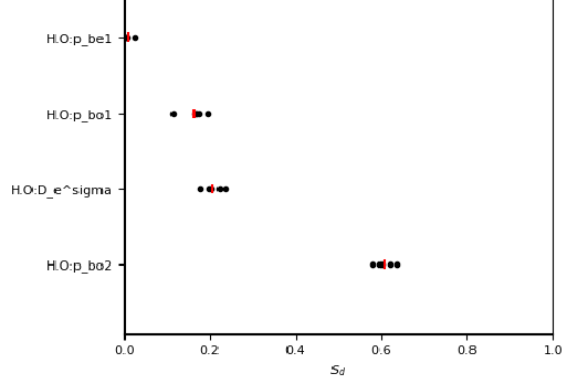
• sensitivity_per_parameter.png is a visual summary of sensitivity values for every parameter and every repeat.

  

• sensitivity_summary.png (and gui_sensitivity_summary.png) are discussed in Graphical results.

• sensitivity_summary.txt is a textual summary of the calculation inputs and sensitivity values for every parameter.

                     HSIC Result
  ==================================================
  Calculation Description:               TrainingSet
  --------------------------------------------------
  No. Factors                                     12
  No. Samples                                    500
  No. Bootstraps                                   5
  Sample with replacement                       True
  Includes reweight calc.                         No
  --------------------------------------------------
  Inputs Kernel                       GaussianKernel
     sigma                                       0.3
  Outputs Kernel           ConjunctiveGaussianKernel
     gamma                                       0.3
  --------------------------------------------------
  Factor Rankings:
       1.                      H.O:p_bo2 0.607±0.020
       2.                  H.O:D_e^sigma 0.207±0.021
       3.                      H.O:p_bo1 0.163±0.026
       4.                      H.O:p_be1 0.008±0.009
       5.                      H.O:p_bo3 0.003±0.005
       6.                      H.O:p_bo4 0.003±0.005
       7.                      H.O:p_be2 0.003±0.003
       8.                      H.O:p_bo5 0.002±0.003
       9.                    H.O:p_ovun1 0.001±0.001
      10.                     H.O:D_e^pi 0.001±0.002
      11.                   H.O:D_e^pipi 0.001±0.002
      12.                      H.O:p_bo6 0.001±0.001
  ==================================================
  

4.4.3.4. Using the results for optimization

The purpose of sensitivity analysis is guide parameter selection for optimization.

Our results suggest that only three parameters have an effect on the loss function.

We have run the optimization version of this tutorial 10 times:

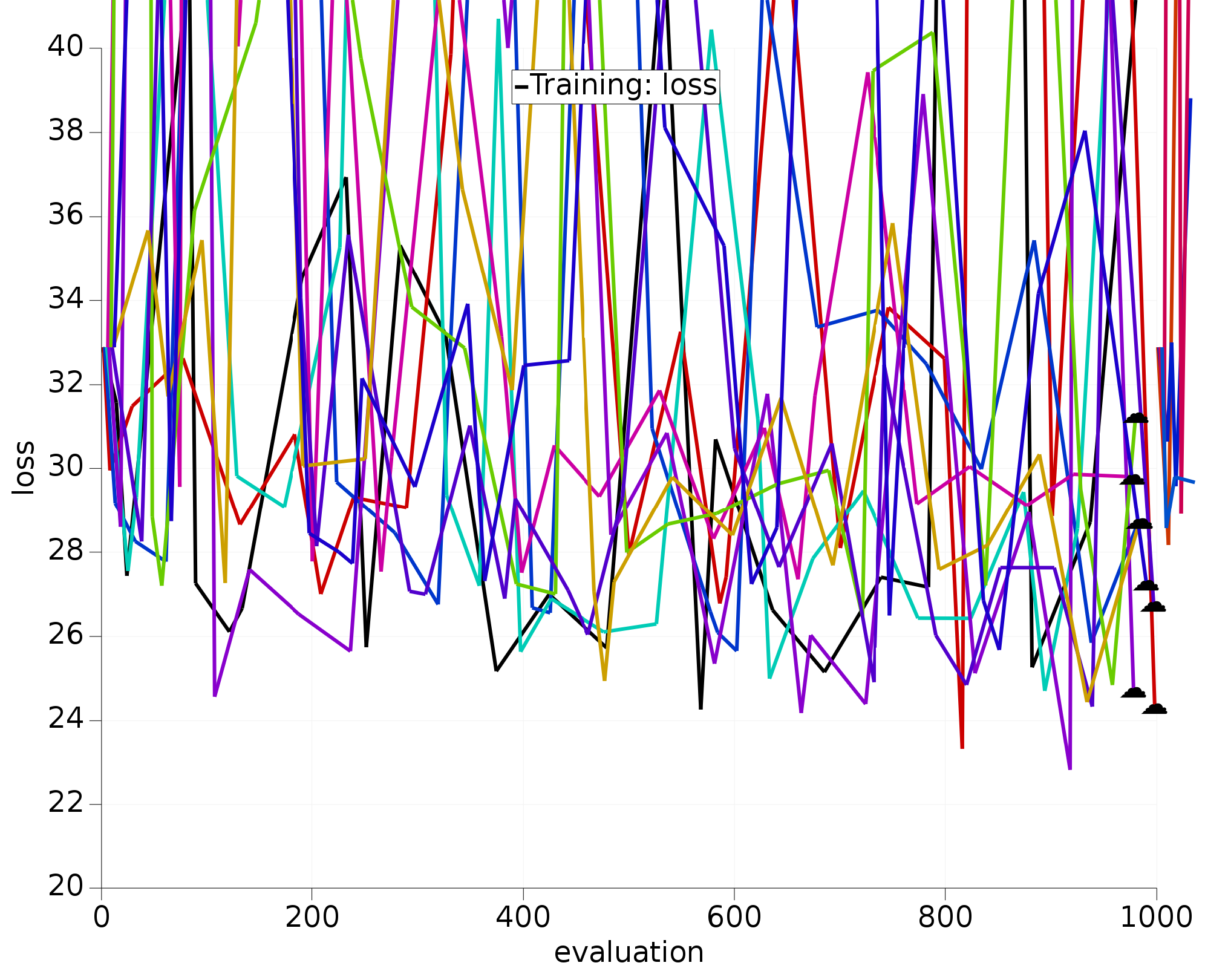
Fig. 4.11 10 optimizations using all 12 H.O parameters.

We have also run the optimization with the exact same settings, but with only the three most sensitive parameters active; also repeated 10 times:

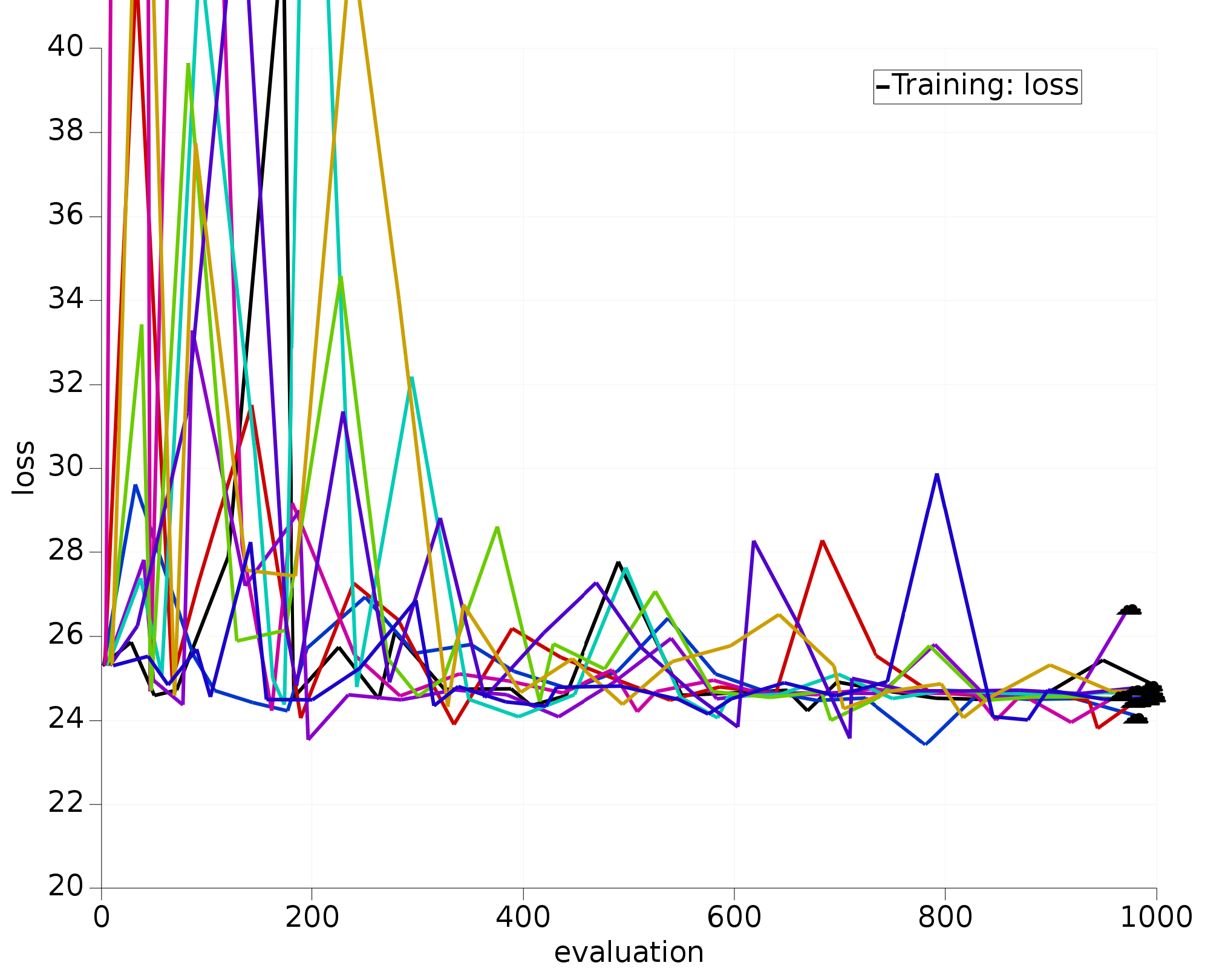
Fig. 4.12 10 optimizations using 3 most sensitive H.O parameters.

The optimizers working only with the most sensitive parameters clearly:

• converge much faster;

• all find same/better loss function values than the 12D optimizers.

See also

To learn about running multiple optimizers at once see Parallel optimizers.

4.4.4. Limits of the sensitivity calculation

There are several factors which affect the accuracy of the sensitivity calculation:

• having a sufficient number of samples is the most important factor, particularly in high-dimension;

• more repeats will provide a more accurate sensitivity average;

• make subsets large enough;

• kernel hyperparameters should not be overly restrictive;

It is also important to be aware of the conditions which invalidate a sensitivity calculation. If any of the following changes are made after a sensitivity calculation, then you should no longer rely on the sensitivity values:

• adding/removing/editing items in the training set;

• changing sigma/weight values in the training set;

• changing job collection settings;

• changing a parameter to in/active;

• changing a parameter range.

Warning

If a modification is small, one might reasonably expect the sensitivity values to remain reasonably unchanged, however, there is no guarantee that this is true. The sensitivity profile might be radically different.

Finally, there is a tradeoff when choosing the number of parameters to optimize. When activating fewer parameters the optimization becomes easier and faster, but, this usually comes at the cost of making the minima worse. This is because there is less flexibility in the potential function to fit itself to all the training data. Worse minima is not always a bad thing. Using fewer parameters can reduce the problem of overfitting.

4.4.5. Some rules of thumb

1. When picking parameters be guided by sensitivity, but consider including several less sensitive parameters in your selection (if their selection makes intuitive sense). For example, in a training set with no π-bonds, do not activate π-bond related parameters but a low sensitivity σ-bond parameter may make sense.

2. Roughly, for a training set with \(n\) items, do not fit more than \(\sqrt{n}\) parameters.

3. For a successful production-quality reparameterization you may need to optimize in several steps: first with very sensitive parameters and then only with moderately sensitive ones.

4. If sensitivities are very imbalanced (a handful of parameters are much more sensitive then the others) consider optimizing in multiple steps or redesigning/reweighing the training set to balance the sensitivities better and make the loss function easier for the optimizers to minimize.

4.4.6. Sensitivity job in Python

In the examples directory, the file sensitivity.py shown below illustrates how to

• run the sensitivity calculation

• create a new parameter interface with only the 3 most sensitive parameters active

• run an optimization job using the new parameter interface

The code below uses the ParAMSResults.get_ordered_parameters() function to extract a list of parameter names sorted by sensitivity. For more possibilities, see the ParAMSResults API.

#!/usr/bin/env amspython
from scm.plams import *
from scm.params import *
import os

def main():
    init() # initialize PLAMS workdir
    examples_dir = os.path.expandvars('$AMSHOME/scripting/scm/params/examples/ReaxFF_water')

    sensitivity_job = ParAMSJob.from_inputfile(examples_dir+'/sensitivity.in', name='sensitivity')    
    sensitivity_job.run()
    # or load a finished sensitivty job using ParAMSJob.load_external:
    #sensitivity_job = ParAMSJob.load_external('plams_workdir/sensitivity/results')

    # create a new interface with top 3 sensitive parameters activated
    new_interface_path = 'top3_activated_interface.yaml'
    create_interface_with_most_sensitive_parameters(sensitivity_job, new_interface_path, N=3)

    # load the optimization job from examples directory but use the new parameter interface
    optimization_job = ParAMSJob.from_inputfile(examples_dir+'/params.in', name='optimization')
    optimization_job.parameter_interface = new_interface_path
    optimization_job.run()

    finish()

def create_interface_with_most_sensitive_parameters(job:ParAMSJob, output_fname:str, N=3):
    """ 
        Gets the N most sensitive parameters from the previous sensitivity job, 
        stores resulting interface in output_fname 
    """
    top_n_sensitive_parameters = job.results.get_ordered_parameters()[:N]
    interf = job.results.get_initial_parameter_interface()
    for p in interf:
        p.is_active = p.name in top_n_sensitive_parameters
    interf.yaml_store(output_fname)

if __name__ == '__main__':
    main()