Bulk Simulation
Periodic boundary conditions can be enabled in order to study the behavior of the bulk layer material under an active current.
Note
You can download the project file
Create Materials
We start by creating the materials that make up the OLED layers. For this tutorial, we will investigate a bulk TAPC material.
Navigate to the Materials tab in the GUI and click on the “+” button above the empty material list. Choose the Transport template to set up a material without excitation processes.
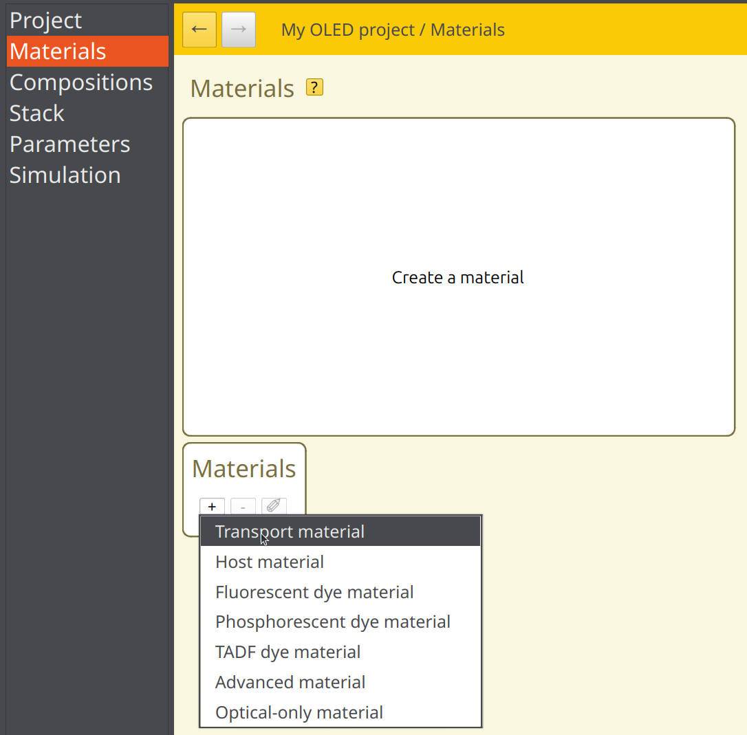
Fig. 17 Create a new material by choosing from template.
This directs you to a material editing page.
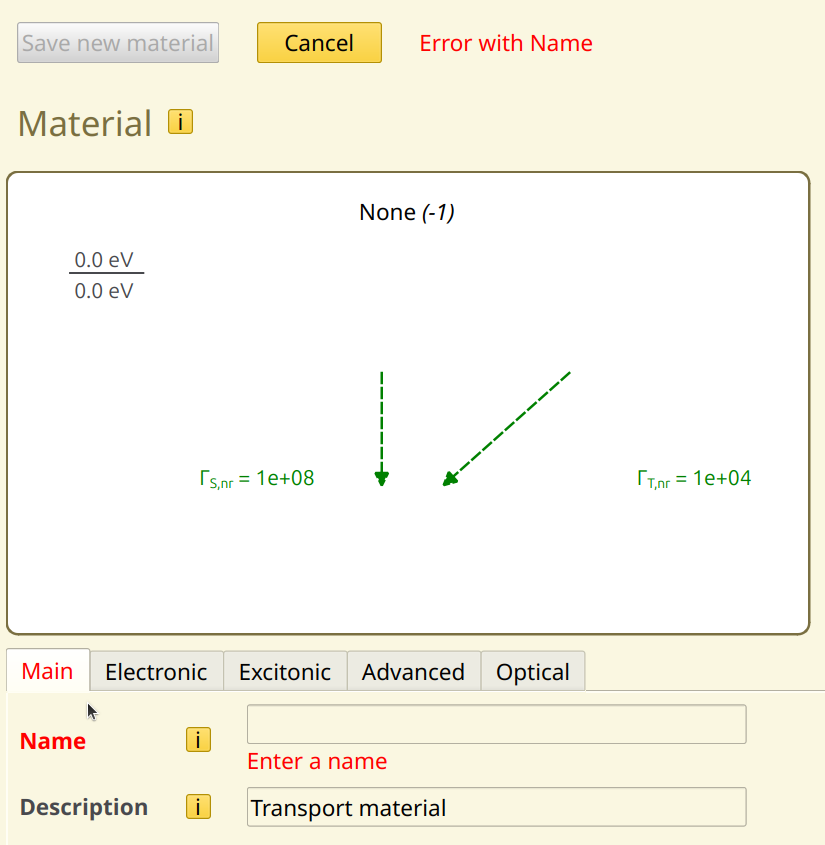
Fig. 18 When creating a new material we see that there are errors.
One important feature is that when editing a material there may be one or more errors. At the top of the page one of those is shown in red. Then below the field with the error is also highlighted in red. On error the “save material” button is disabled. In this case the error is easily fixed by entering a name, for instance TAPC.
The Electronic tab specifies the parameters for the polarons (electrons and holes). For this tutorial, we will use a HOMO level of -5.5 eV and a LUMO level of -0.96 eV.
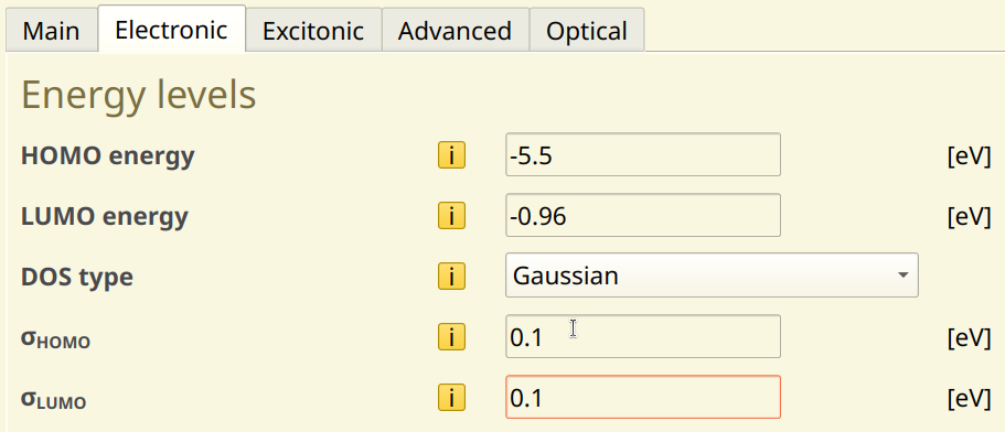
Fig. 19 Polaron settings page for the new material
The DOS type is used to introduce variations in the energy levels between gridpoints. Due to the amorphous nature of typical OLED materials, the molecular environment differs throughout the layers. These environmental differences affect the inter-molecular interactions, resulting in a distribution of energy levels.
Here, a Gaussian distribution will be used to model this effect. Set both the standard deviations to 0.1 eV. We will leave the transport parameters at the default for now.
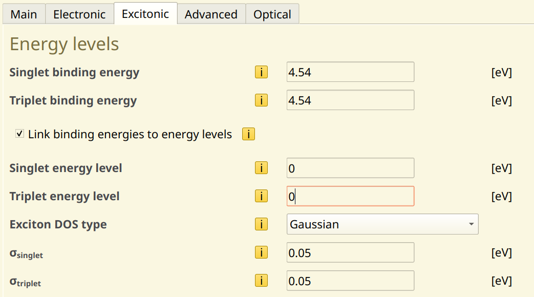
Fig. 20 Exciton settings page for the new material
The Excitonic tab specifies parameters for the excitons (singlets, triplets) and the excitation processes. As we will not be modeling excitons in this tutorial yet, simply set the singlet and triplet energy levels to 0. You can now save the material.
Saving the material
When saving the (new) material also a pure composition will be made. You can see it in the Compositions page and also the Project page.
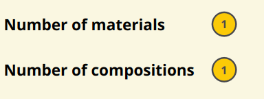
Fig. 21 Feedback on the Project page.

Fig. 22 The pure composition is also listed in the Compositions page.
If you select the pure TAPC composition (double click in the compositions list), you will see that it has a mole fraction of 1 for the TAPC material that we just created.

Fig. 23 Pure compositions are automatically created for new materials,they contain only one material with a fracion of 1.
Saving the project
When you save a material (or composition) this merely aplies the changes to the project. So it is a good idea to save the project file as well. (File -> Save). The first time a file dialog will open you can name it bulk in any convenient directory. Bumblebee projects are saved with the .bee extension.
Create a Stack
After defining the materials, we can now create an OLED stack by defining the layers. Here, we will be using only a single layer in order to model the bulk material behavior.
Navigate to the Stack page in the GUI. As before, provide a name for the stack. Then click on the “+” button in the Layers table. In the table you can edit directly the thickness and can set it to 50 nm. Then press Save stack
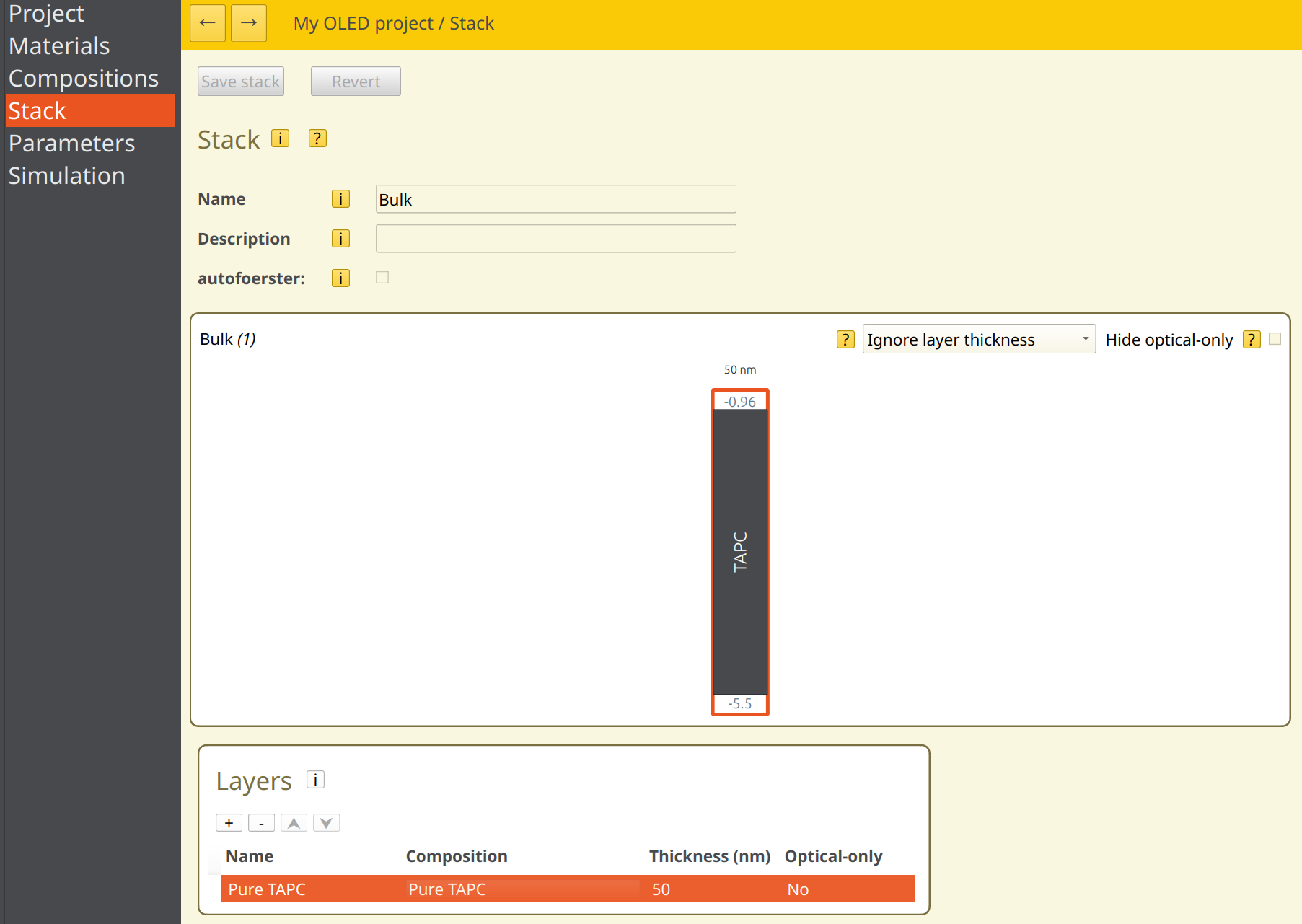
Fig. 24 Make sure the page looks like this. A diagram of the stack is shown, being very simple for this stack.
You can also change directly the name of te layer and the composition (via a menu popup), but here there is only one composition and the automatic values are fine.
The remaining (empty) tables of the (lengthy) Stack page relate to the excitonic processes, so we can leave these alone for now.
Create a Parameter Set
Having created an OLED stack, we will now configure the simulation settings. Navigate to the Parameters page and push the New from preset button.
You will be prompted to select a template. As we are modeling a bulk material, select the Periodic Box. This will automatically configure some of the presets required for the bulk simulation.
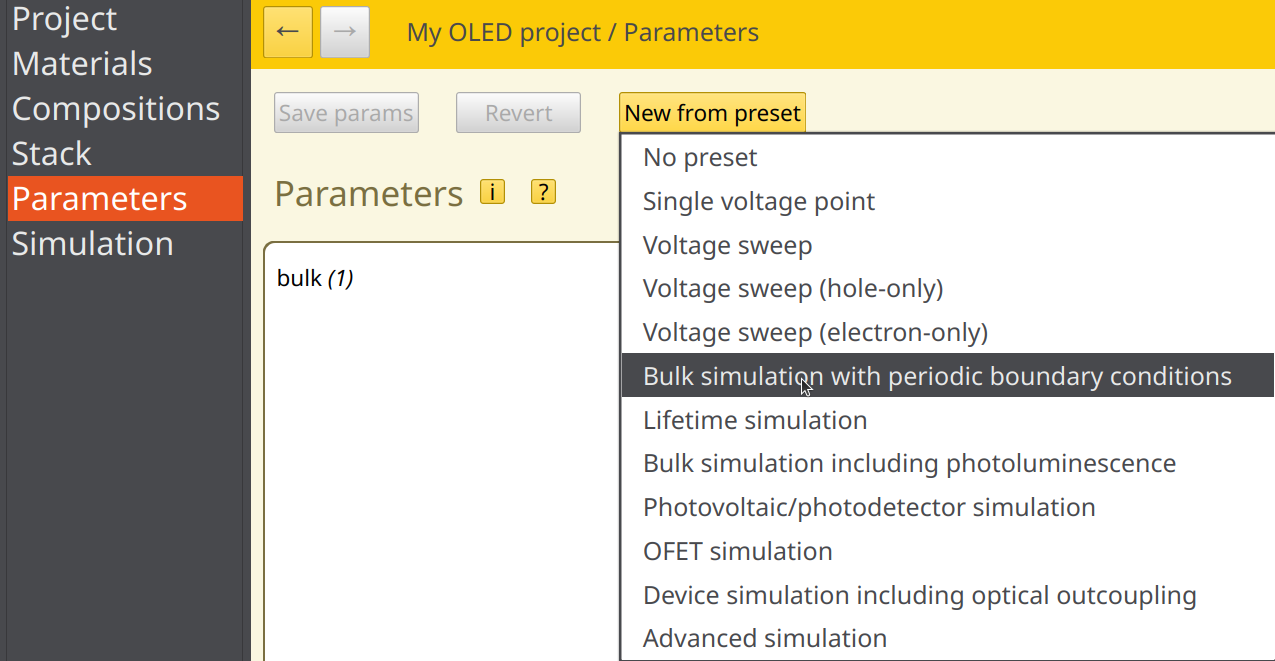
Fig. 25 Selection of the bulk preset
Device Settings
In the Main tab, provide a name for this parameter set.
In the Physical Parameters section of the Main tab, we can set the device voltage. We will use 1 V for this simulation. Keep the temperature at 300 K. The relative permittivity is used to set the effective permittivity of the device (i.e. for all the layers in series). For now, we will use a default value of 3.
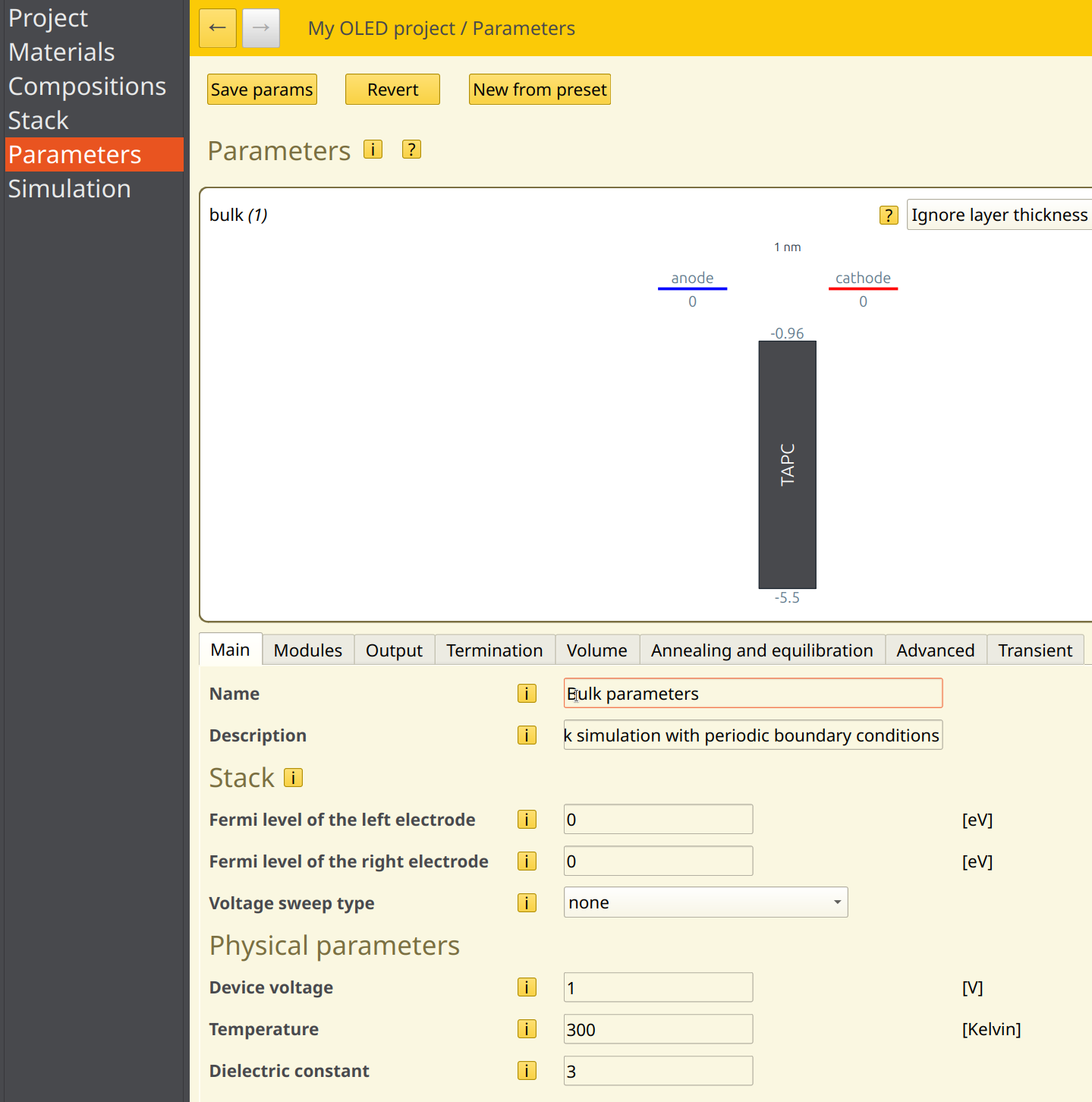
Fig. 26 The Parameter page for this tutorial
Finally, press the ‘Save params’ button to apply the changes to the project.
Simulation Volume
Simulation volume settings are provided in the Volume tab. The periodic boundary conditions should have been enabled by default when using the Bulk simulation template.
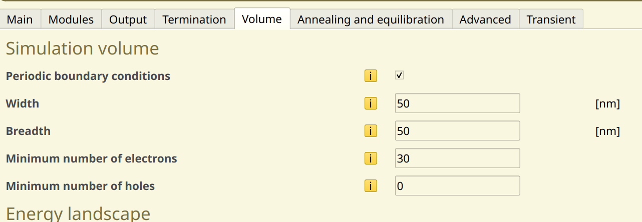
Fig. 27 Volume settings for a parameter set
The number of sites determines the simulation grid and sets the size of the modeled surface area of the cell. We will use the default of 50 nm in both directions.
Because we are modeling the bulk of the device using periodic boundary conditions, this means that the electrode contacts are not included in the simulation grid. A fixed number of polarons will therefore be used to investigate charge transport. We will use a single polaron type for this tutorial by setting the number of electrons to 30 and the number of holes to 0.
Simulation Duration
The Termination tab specifies the duration of the simulation.
As Bumblebee determines the device performance through stochastic sampling, it is important that a sufficient number of steps is allowed in order to provide accurate statistics. This can be achieved in 2 ways:
Increase the number of steps in the simulation
Perform multiple simulations in parallel and collect the results (this can be enabled during the job submission step)
For this tutorial, we will set the number of simulation steps to 30.000.000. This determines the maximum number of steps that the simulation will go through. Additional convergence criteria can be specified in this tab to allow early termination. These can be left off for now.
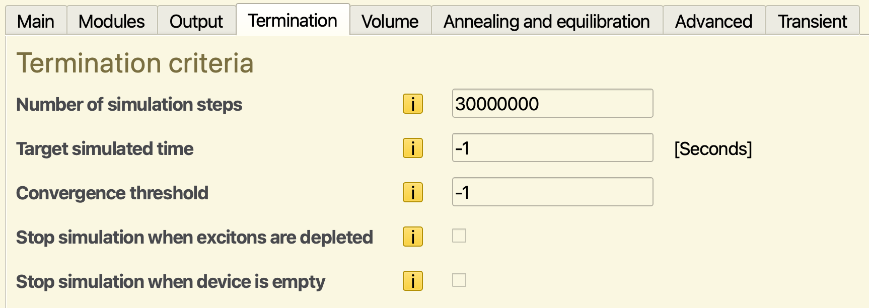
Fig. 28 Termination criteria
Output Settings
The Output tab allows specifying the frequency with which simulation results are reported. This frequency is set separately for 2 types of files:
The report interval determines how often the simulation summary and log files are updated
The output interval determines updates to the remaining output files
Writing output to a large number of files can slow down the simulation significantly. For this reason, the output interval is often taken to be larger than the report interval. Individual output files can also be enabled or disabled manually in the Output tab to reduce the cost of writing files.
For this tutorial, we will set a report interval of 5000 steps and an output interval of 1.000.000 steps.
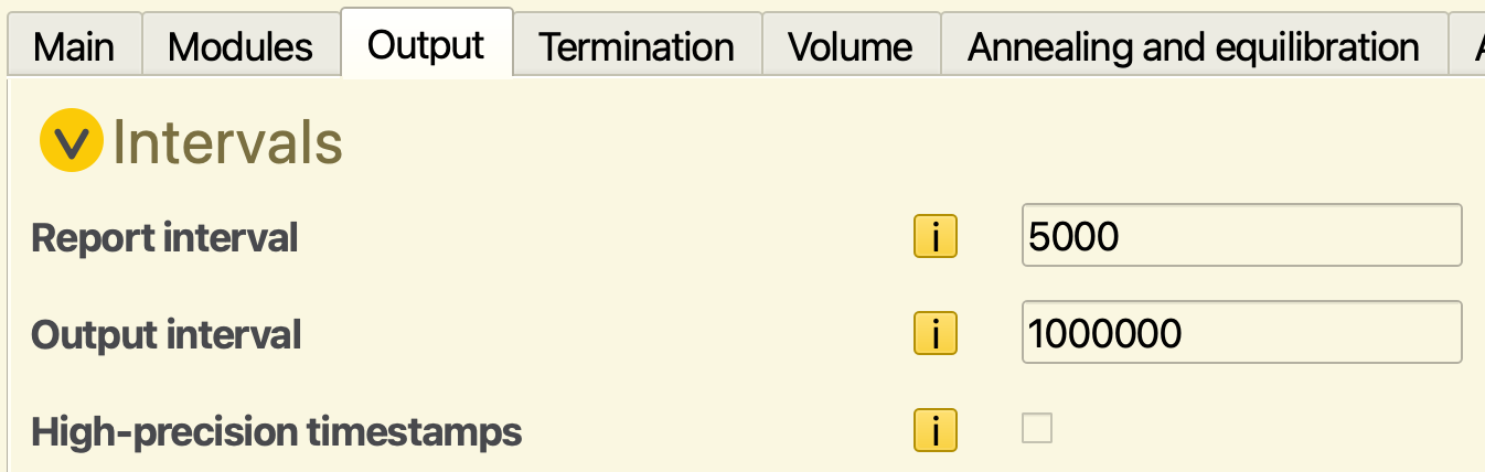
Fig. 29 Output settings
Finally, press Save params, to apply the changes to the project.
Starting the Simulation
Given the stack and parameters, it is common to perform many independent calculations. So-called trajectories (or disorder instances) are used to build statistics, via random initial conditions. Bumblebee will automatically collect sample data from each simulation and include this data in the device statistics.

Fig. 30 Trajectories and Sweeps can be defined on the Simulation page
By setting the First/Last trajectory to 1/2 we select only 2 trajectories in order to illustrate this process (without using too many resources). To obtain better statistics, you can increase the number of trajectories here, or the simulation time in the parameter set. Note however, that this will also increase the computational cost of the simulation.
The sweep parameters will not be used for this tutorial.
Save the project (File->Save) and press run (File->run). You can also start the job from AMSjobs.
Monitoring the Simulation
Select BBresults from the SCM menu.
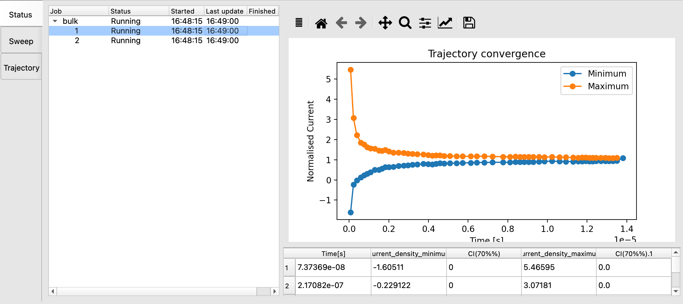
Fig. 31 Progress of a running bumblebee job from BBresults
The Status tab shows the simulation convergence. Many other graphs are also available for a running job.
BBresults also offers options to request termination of trajectories, sweeps.
Fixme: Simulation Output
After the simulation has finished, you can view the results in the Simulations tab. Selecting a simulation will bring you to the Overview tab. The Sweeps tab lists the associated jobs. The job progress can be viewed in the Jobs tab.
The simulation output is collected in the Reports tab. The web interface handles automatic visualization of various results. An overview of the visualization options is collected in the manual.
The Single Box tab shows the results for each job. This allows you to analyze the individual trajectories. The Multibox tab provides the aggregate results obtained from collecting the data from multiple boxes. Navigate to the Files tab if you want access to the raw simulation output.
Tip
It is possible to add additional boxes to the simulation in order to improve the statistical estimates, even if the simulation has already been completed. Select the simulation and navigate to the Sweeps tab. Select the Add Sweep option to increase the disorder instance range. This will submit additional jobs to the server. Simulation reports are updated as these jobs complete.