Parameter Screening: Voltage Sweep

Simulation parameters can be screened in order to study device performance under different conditions, or to search for desired material properties.

Create Materials

We start by creating the materials that are used in the stack.

• NPD has a HOMO energy of -5.45 eV and a LUMO energy of -1.4 eV

• mCBP has a HOMO energy of -6 eV and a LUMO energy of -1.5 eV

• Ir(dmp)3 has a HOMO energy of -5 eV and a LUMO energy of -1.7 eV

Tip

If you have never created materials before, take a look at the start of the bulk tutorial.

For this tutorial, we will focus on charge transport only. The Transport template can be used when creating new materials via the “+” buttons in the Materials table. We will use a Gaussian DOS with a standard deviation of 0.1 for both polarons (see the Electronic tab where you also enter the HOMO and LUMO levels). Excitonic processes will be omitted for now.

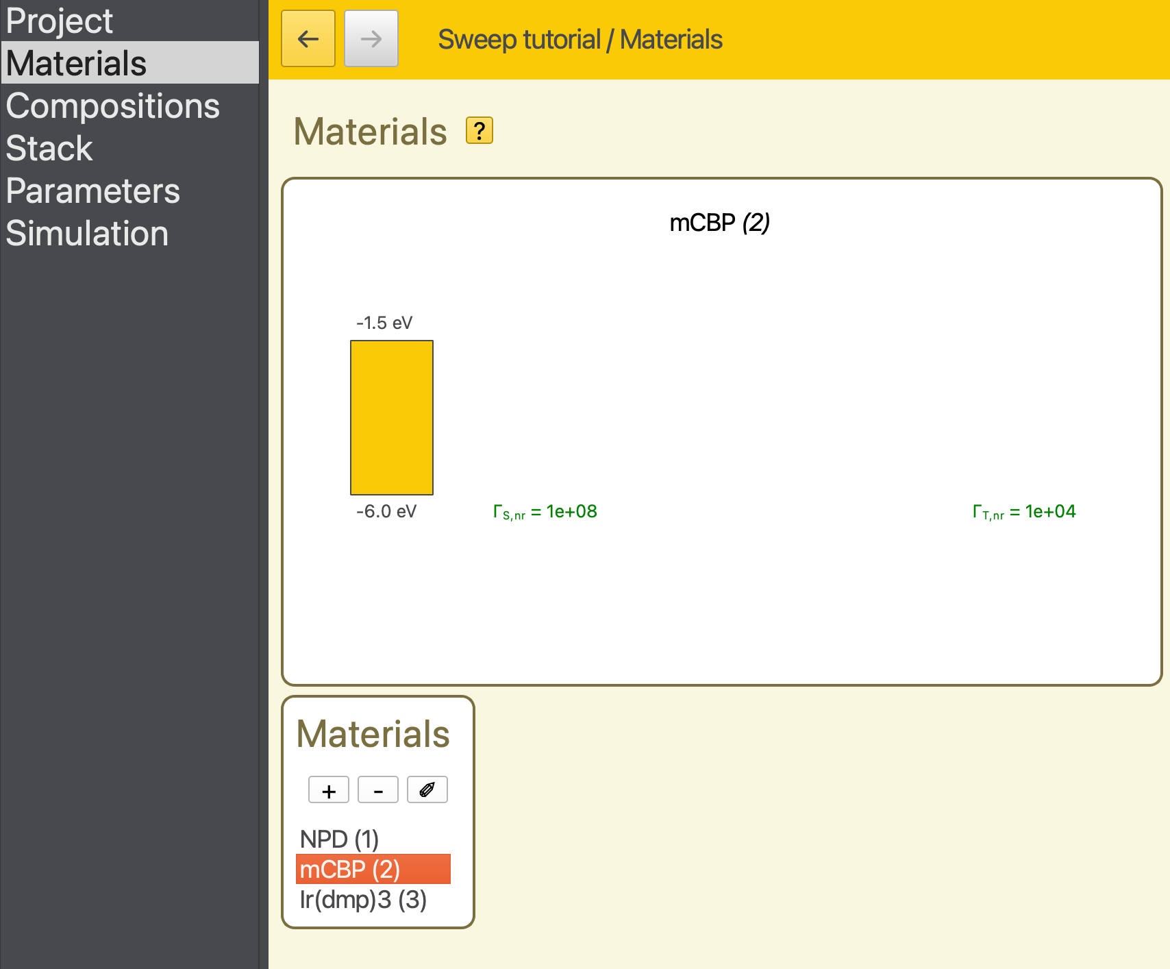
Fig. 32 The material list is convenient to quickly see the HOMO/LUMO levels of the materials, under/above the orange box in the material diagram. Here the second material is selected in the Materials table.

Create Compositions

Navigate to the Compositions page to access the compositions that make up the device layers. Pure compositions for each of the compounds have already been created.

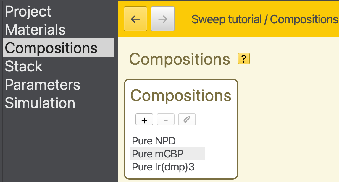
Fig. 33 The pure compositions are already on the Compositions page.

In addition, we are going to create a new host-guest mixture. Click on the “+” button in the Compositions table, leading to a Composition editor page.

We will create a mixture of 0.9 mCPB and 0.1 Ir(dmp)3. To add a component to the mixture, simply click the “+” in the Fractions table. Then you can directly edit in the table the material and the fraction.

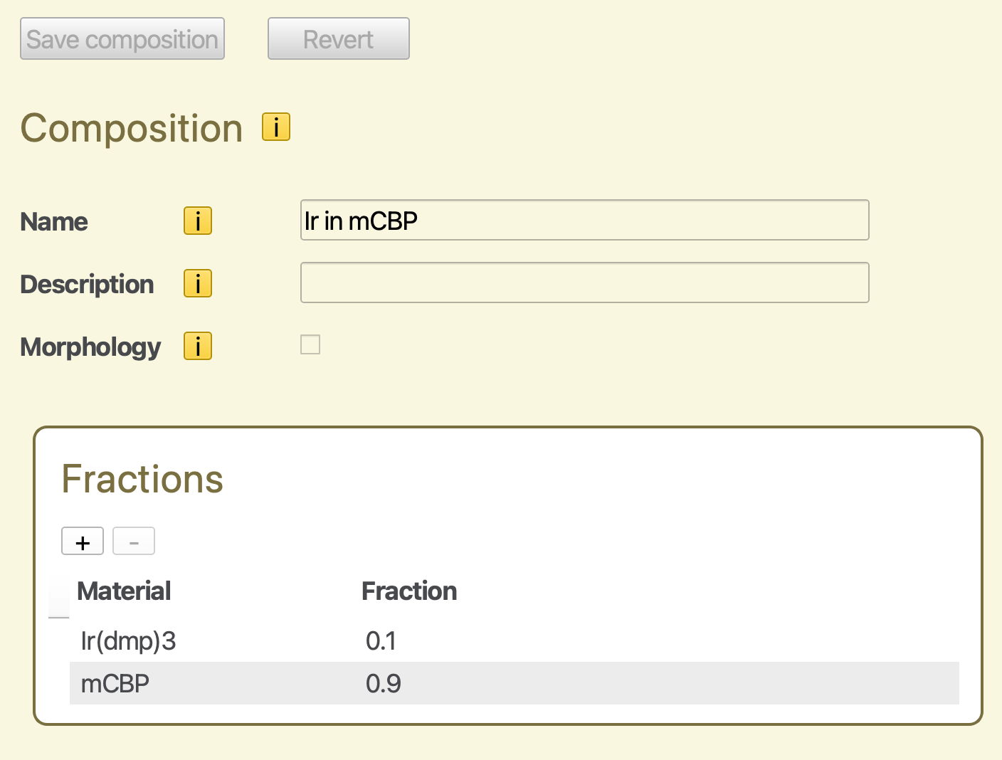
Fig. 34 Mixed composition for a host-guest system

Click the Save Composition button to add it to the project. You can check the Compositions page that there are now four compositions. When you are satisfied save the project.

Create a Stack

We will create a stack using 3 layers. The outer contact layers are composed of pure NPD. The inner emitter layer contains the host-guest mixture defined earlier.

• Create a 10 nm NPD layer

• Create a 60 nm layer containing the mCPB-Ir(dmp)3 mixture

• Create another 10 nm NPD layer

You will end up with an 80 nm stack.

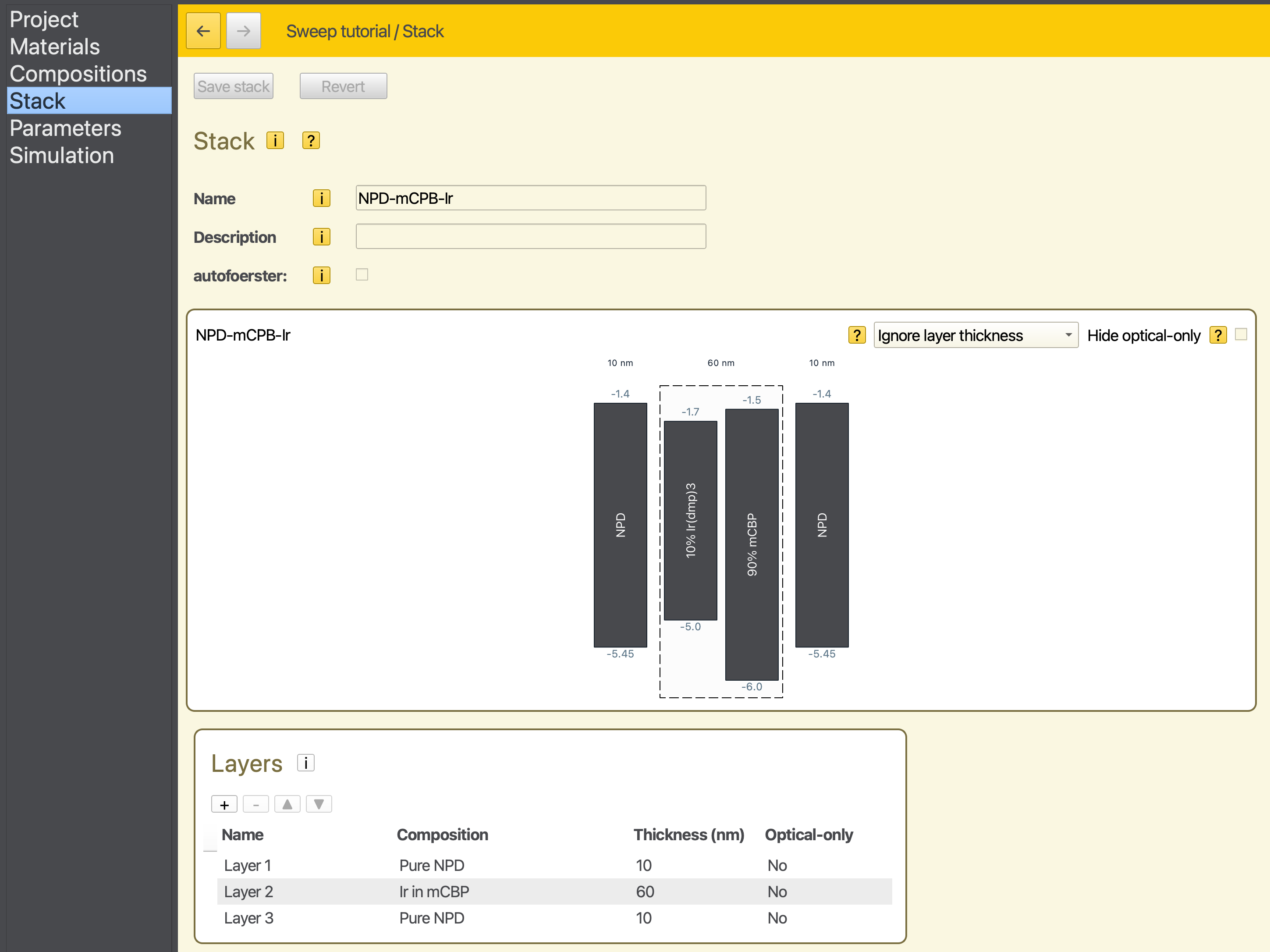
Fig. 35 The final Stack page

The diagram is intereractive. Try ctr+click on a material of composition. This brings you to a material or composition page. Use the back navigation button to return to the stack. You can also change the stack visualisation from from Ignore layer thickness to other values.

Create a Parameter Set

For this simulation, we are interested in investigating the device performance at different voltages. Click on the New from preset button and select Voltage sweep

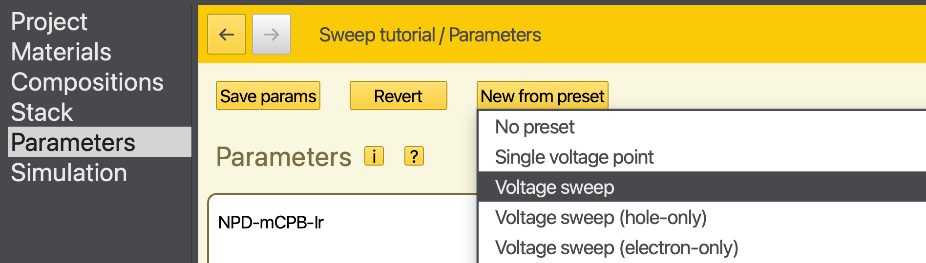
The voltage will be set as part of the parameter screening and does not need to be chosen at this step.

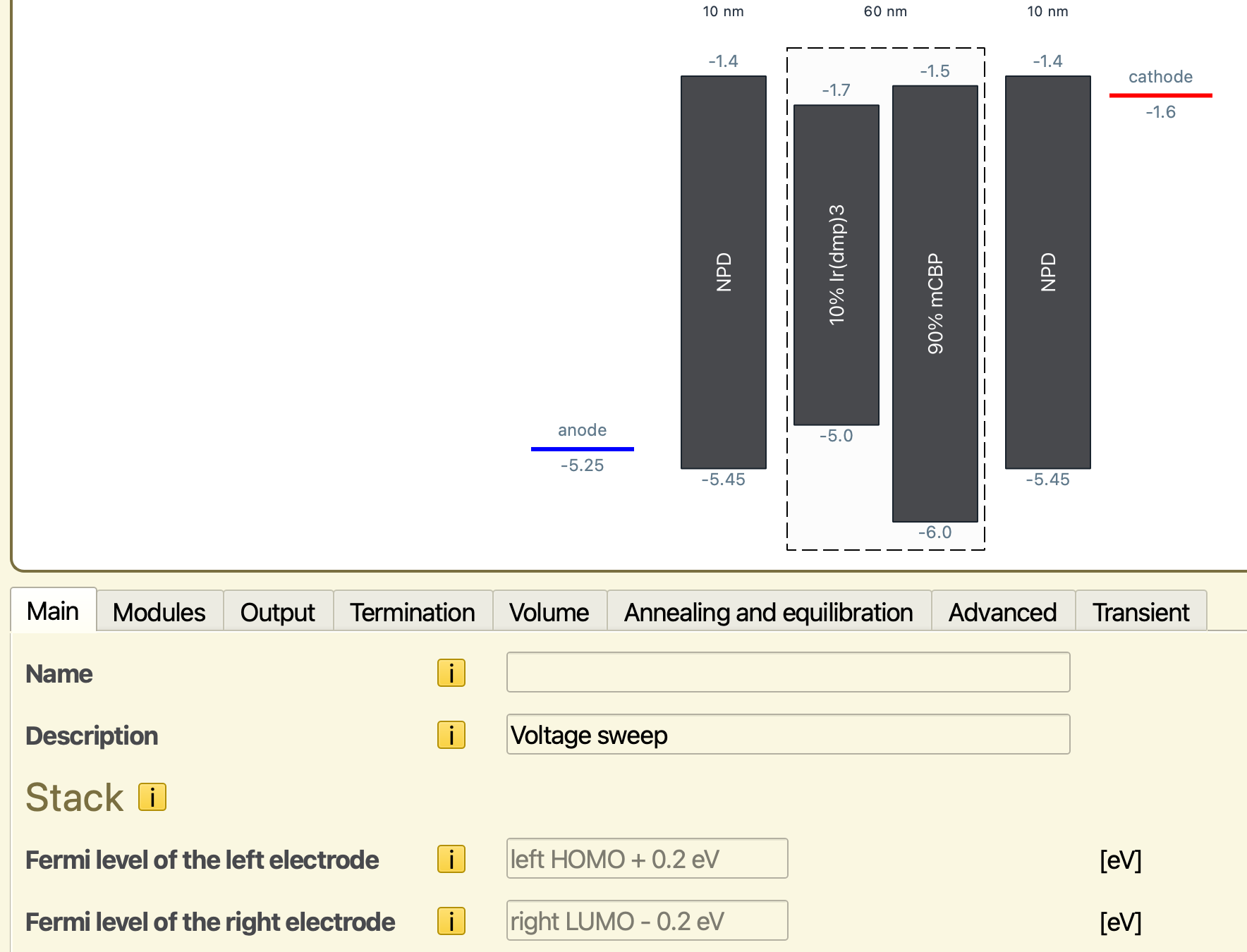
Fig. 36 Electrode contacts are configured automatically to include an exchange barrier

The Fermi levels of the electrodes are automatically matched to the material parameters. These levels can be adjusted to those of the external contacts. We will use an electrode energy level of -5.25 at the anode and -1.2 at the cathode. By using an energy barrier of 0.2 eV compared to the NPD polaron energy levels, we are reducing the rate of polaron exchange processes with the electrodes. This biases the kMC simulation, increasing the number of samples that contain transport processes compared to electrode exchange.

Note

Care should be taken that this artificial barrier does not affect the device statistics. This can be achieved by analyzing the change in device properties when varying the barrier height. Because electrode exchange processes are localized at the edges of the device, a single-layer simulation can be used to perform these screenings, significantly reducing the simulation costs.

Note

When operating under high currents, the device sensitivity to the barrier height may become voltage-dependent. Make sure to verify the validity of your data at both extremities of the investigated voltage range.

The Modules tab allows you to enable different processes that are allowed to occur during the simulation. As we focus on polaron transport for this tutorial, all modules can be disabled (being the default).

For the tutorial we will set the number of simulation steps to 1.000.000 in the Termination tab. On the Output tab, we set the report interval to 10.000 and the output interval to 100.000. Press the Save params button to bring the changes to the project.

Note

For production runs set the number of simulation steps to 1.000.000.000, the report interval to 100.000 and the output interval to 1.000.000.

Starting the Simulation

Navigate to the Simulation page. For tutorial purposes, we can set the disorder instances to 1, i.e. use only one trajectory.

Parameter screenings can be specified as part of the simulation setup. The screening allows evaluation of the device behavior for different parameter values. Aside from the sweep parameter, all other conditions will remain unaltered from the default parameter set.

The screening values are obtained through linear interpolation. Minimum and maximum values for the screening parameter are selected and the total number of screening steps is chosen. A uniform step size between parameter values is calculated.

Fig. 37 Voltage sweep setup in the simulation settings

For this example, we select voltage as our screening parameter. The minimum and maximum voltages are set to 1 and 5 V respectively. By choosing 3 voltage steps, this will prompt the screening to perform simulations at 1, 3 and 5 V. A preview of these screening conditions is shown.

Note that the number of disorder instances is applied to each screening step. The default of 5 disorder instances would therefore yield 3x5 independent jobs. By using only a single disorder instance, the number of simulation jobs is limited to 3.

Now save the project and run it.

Simulation Output

Open the results with BBresults. Quite obviously the results are not converged with this short simulation. But we can already see meaningful physics

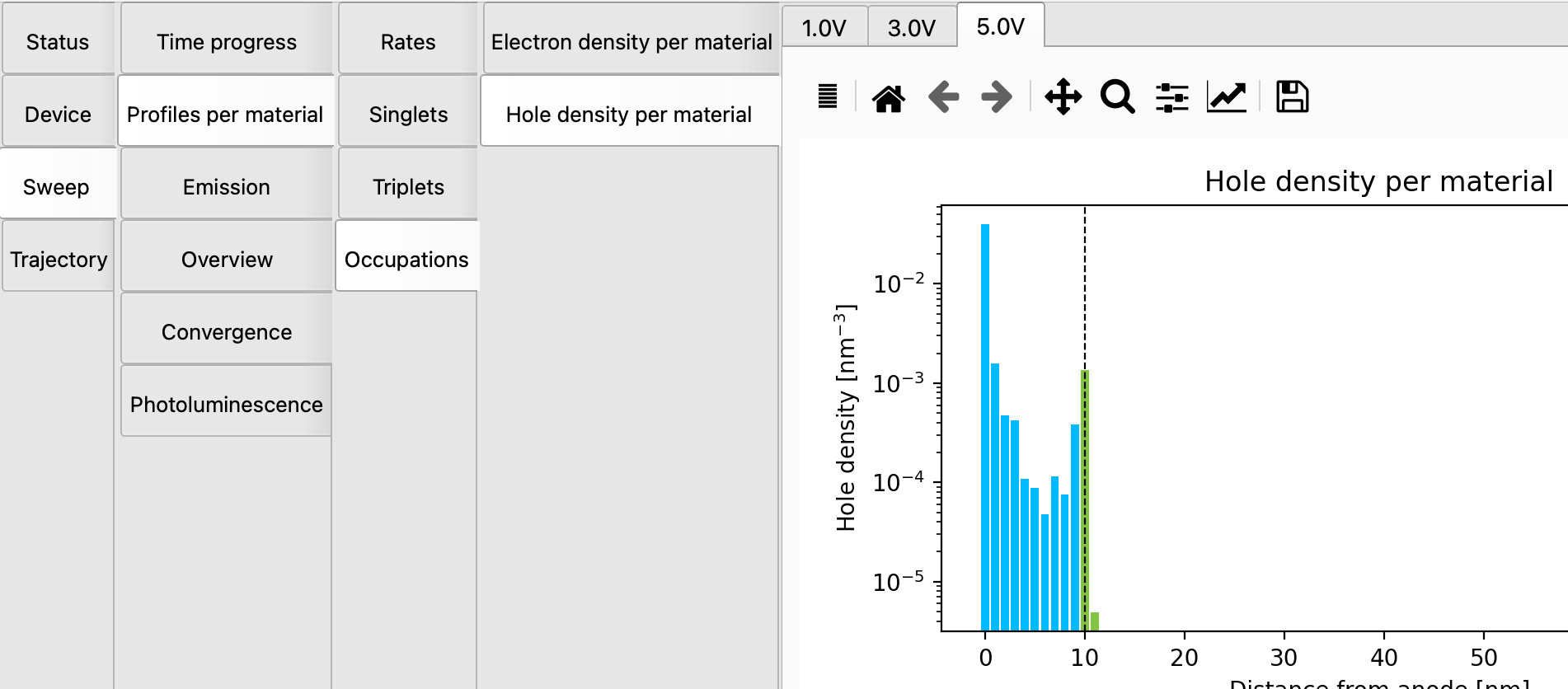
Fig. 38 The hole density per material at 5.0V. Holes start appearing in the middle layer. At lower voltages (click on 3.0V for instance) the positive holes are restricted to the left transport layer (close to the negative anode), and hence are NPD material.

Current-voltage characteristics can be viewed in the Device -> Overview -> Performane section. In this case there is no current for the sampled voltages, due to the short sampling time.

Extending the simulation time

As can be seen from the trajectory convergence plots, the chosen number of simulation steps was way too small, the minimum and maximum being far apart. Look at the time in the trajectory convergence plot, that should be about 7e-7 seconds. An easy way to double that time is by choosing in BBresults “Simulation -> Extend trajectories”. This opens AMSjobs with the job selected that you can run. When it is finished the time should extend to 1.6e-6 seconds… and the results are still not nearly converged. Extending once more makes that about 2.4e-6 seconds.

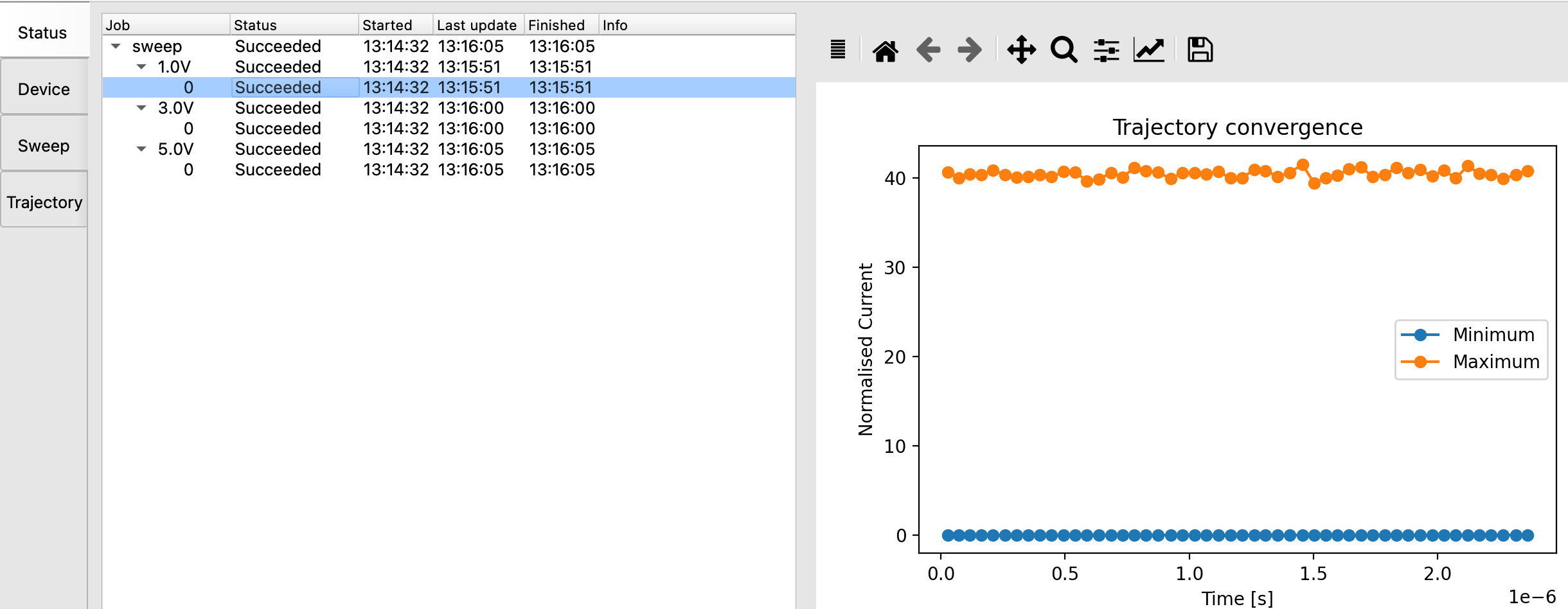
Fig. 39 The trajectory at 1.0V is still not converged after extending the trajectory twice. The trajectory at 5.0V shows much more progress. Converging low voltage trajectories takes longer.

Adding screening/sweep points

Say that you want to screen on a finer volt mesh. Use Simulation -> Add sweep points. In the dialog you can enter that you want to sweep from 1.0 to 5.0 V using 5 points. This will add two new screening points (2.0 and 4.0V).

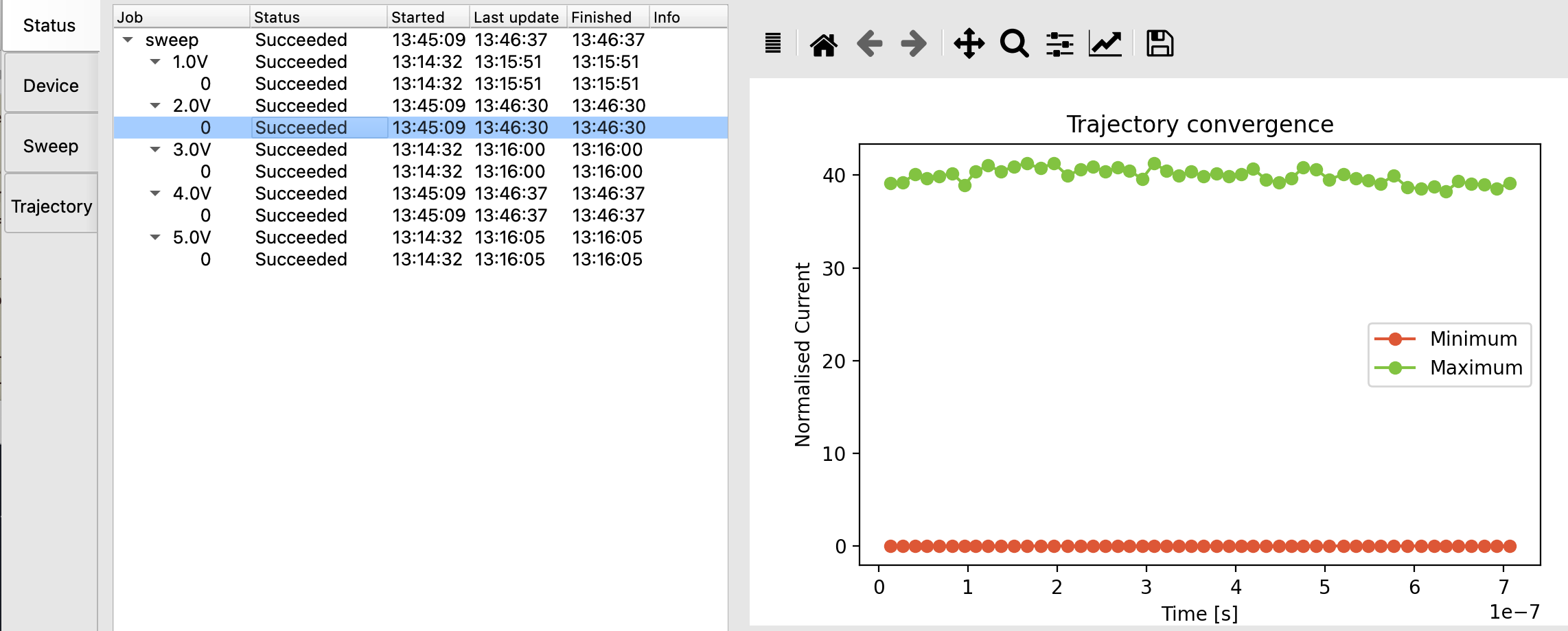
Fig. 40 Convergence plot for the newly added trajectory at 2.0V. Observe that the simulation time corresponds to the original setting in the project. The trajecories for 1.0V, 3.0V, and 5.0V are unchanged (and have a longer sampling time)