GUI tour: UV/Vis spectrum of ethene
In this tutorial you will first construct an ethene molecule and optimize its geometry.
Next you will perform an excitation energies calculation using ADF. The results will be examined using AMSlevels, AMSdos, AMSspectra and AMSview. The use of the KFbrowser is also shown.
Finally you will run an excited state geometry optimization and check its results.
Create your ethene molecule
First we construct an ethene molecule, and pre-optimize its geometry:

 → Double (or use the shortcut: press the ‘2’ - key)
 to pre-optimize
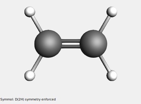
 to symmetrize the structure (it should be D(2H))
Your ethene molecule should look something like this:
Note
Starting from the 2020 release, ADF does not automatically symmetrize and re-orient the molecule.
If your molecule is symmetric and you want to make sure that the highest possible symmetry is used, you should first symmetrize your system with
Optimize the geometry
The next step is to optimize the geometry using ADF:
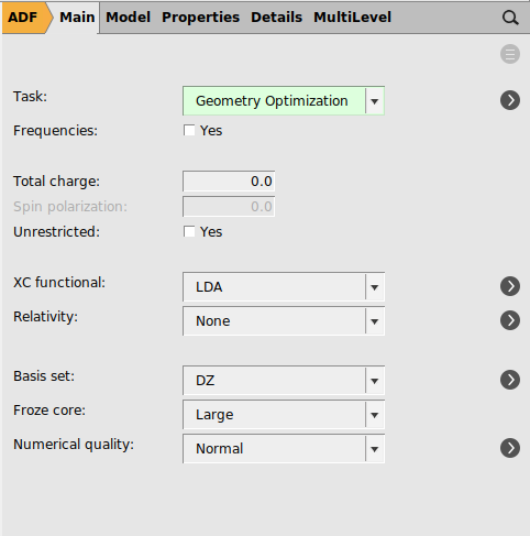
With the proper options selected, now run ADF:
Now ADF will start automatically, and you can follow the calculation using the logfile that is automatically shown.
Calculate the excitation energies
Select calculations options
To set up the calculation of the excitation spectrum:
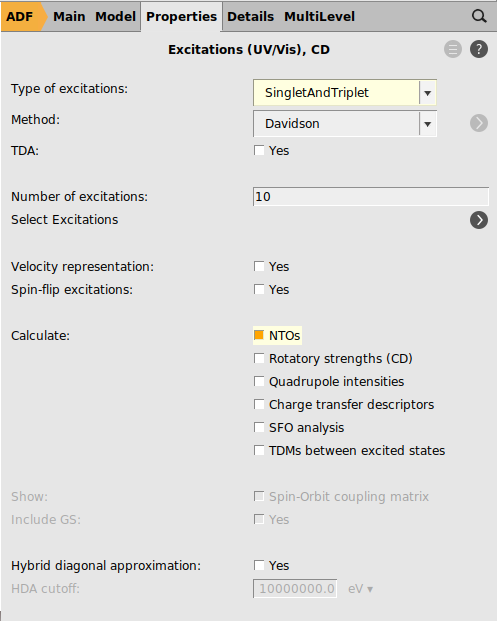
For the tutorial this set up is fine, normally you would also need to select an XC potential and Basis set that gives better results.
Run the calculation
Now everything is ready to run the excitation energies calculation with ADF. Before running we will save the current input in a different file:
Results of your calculation
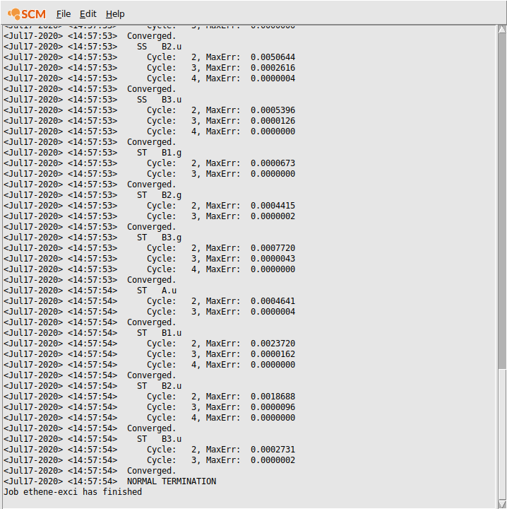
Logfile: AMStail
The logfile shows you that the calculation has finished, and that indeed the excitation code has been running (your output may look slightly different):
Energy levels: level diagram and DOS
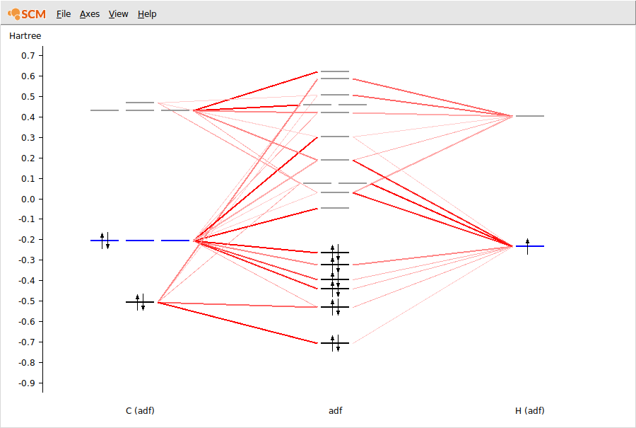
In this level diagram you can see that the HOMO and LUMO consist mainly of carbon p orbitals. It is also easy to see what orbitals the hydrogens take part in.
Tip
You can drag the vertical columns around (the final MOs and the fragments) to get a clearer diagram if needed. Click and drag in the name (at the bottom) to do this.
Note that the carbon and hydrogen stacks show all carbon and hydrogen atoms at once: they show the fragment type. AMSlevels can also show the individual fragments but when using atomic fragments you will get too many fragments. In this particular case symmetry is used, and since there is only one symmetry unique carbon atom and only one symmetry unique hydrogen atom you still would see only one stack per atom type.
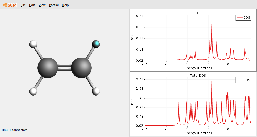
In these plots you can see that the partial DOS for the hydrogen atoms have no contribution to the HOMO. By right clicking on an atom you can also show partial DOS graphs with contribution from selected atoms and selected L-values only.
Excitation spectrum: AMSspectra
AMSspectra will start and show the calculated excitation spectrum.
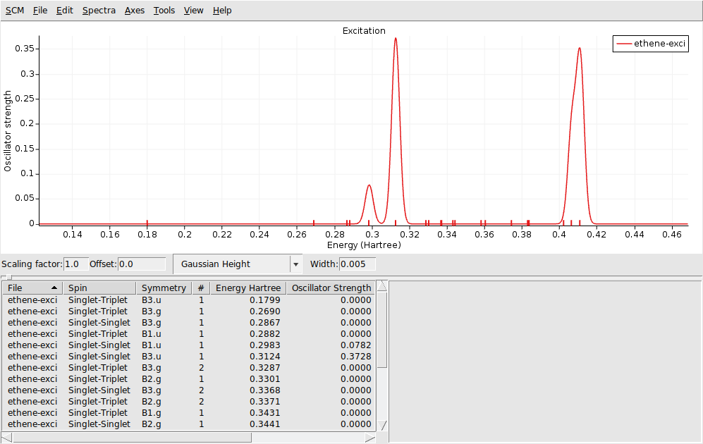
In the window below the spectrum you will find a table with information. You can get more information by selecting one of the entries (or click on the peak in the spectrum):
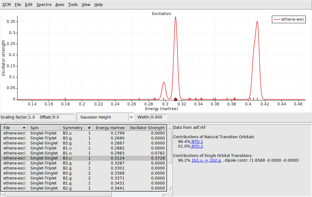
The composition of the excitation in terms of orbital transitions is listed on the right side. In many cases you can visualize relevant orbitals or NTOs with AMSview by clicking on them in the window on the right. The active items are visually marked. You can rotate the view by left-clicking and moving your mouse.
1b1.u -> 1b2.g (with the highlighted orbitals)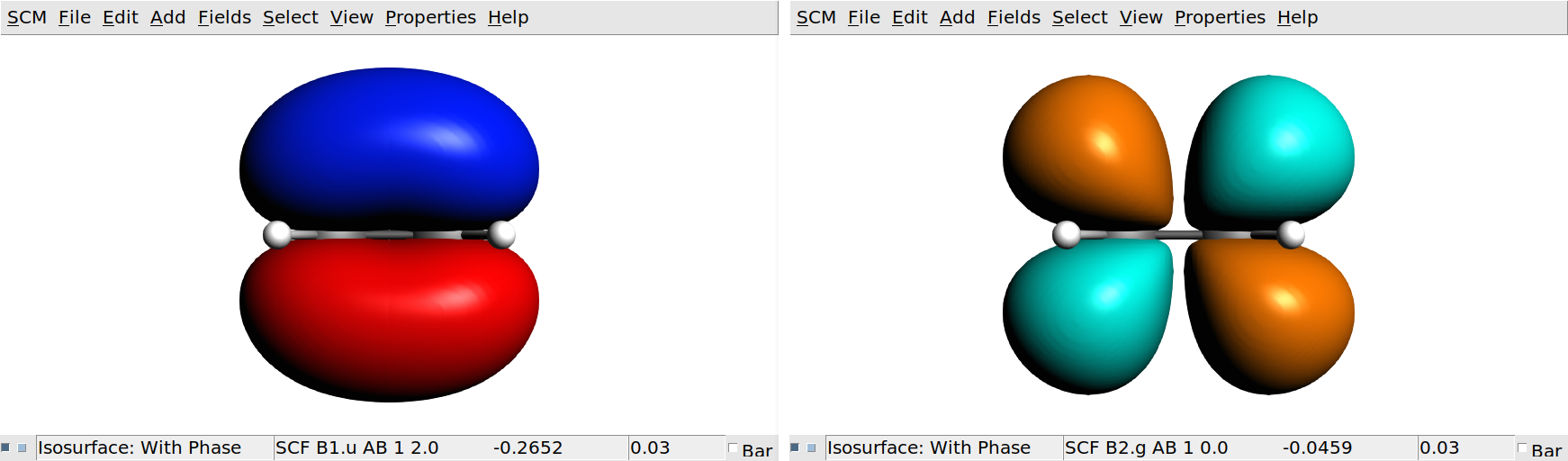
Orbitals, orbital selection panel: AMSview
We will now use AMSview to examine the orbitals. Not just one, but have a look at many of them. To do that AMSview has an ‘orbital selection’ panel.
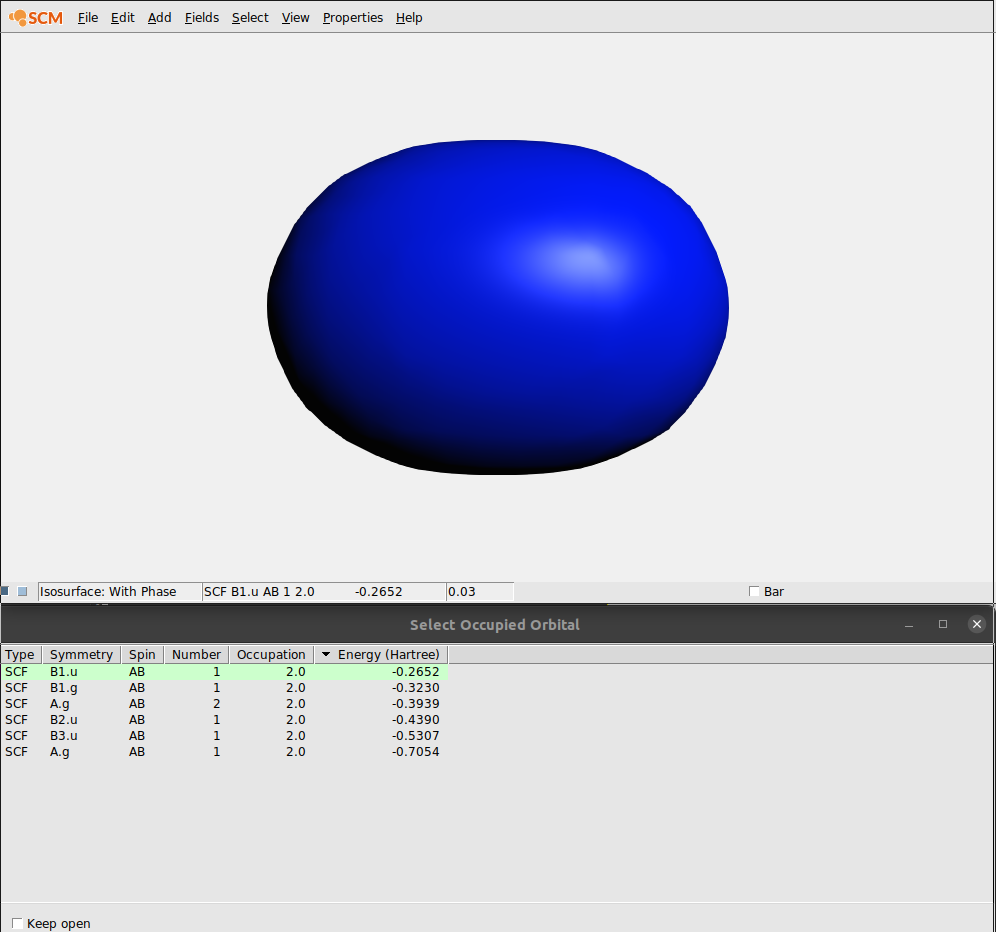
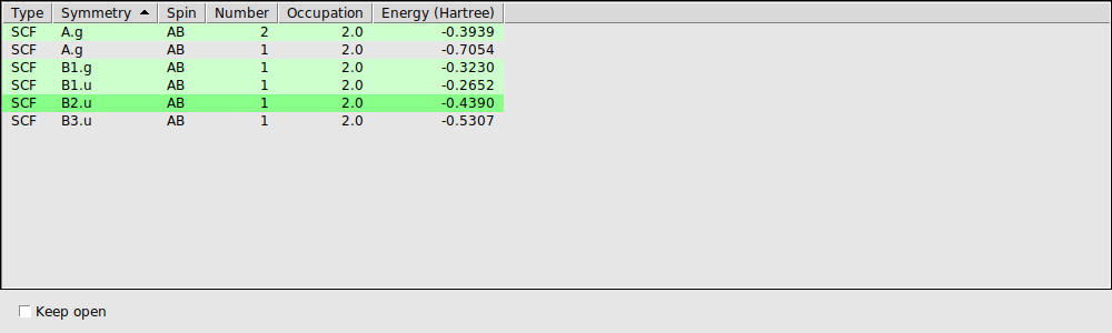
In the ‘Select Occupied Orbital’ window you can select the orbital that you want to see. Note that the currently visible orbital is highlighted using a dark green background.
When you click the first time on an orbital, its values need to be calculated and then the orbital is shown. When you click for a second time on an orbital in the list, it has already been calculated (indicated by the light green background color). And thus it shows immediately.
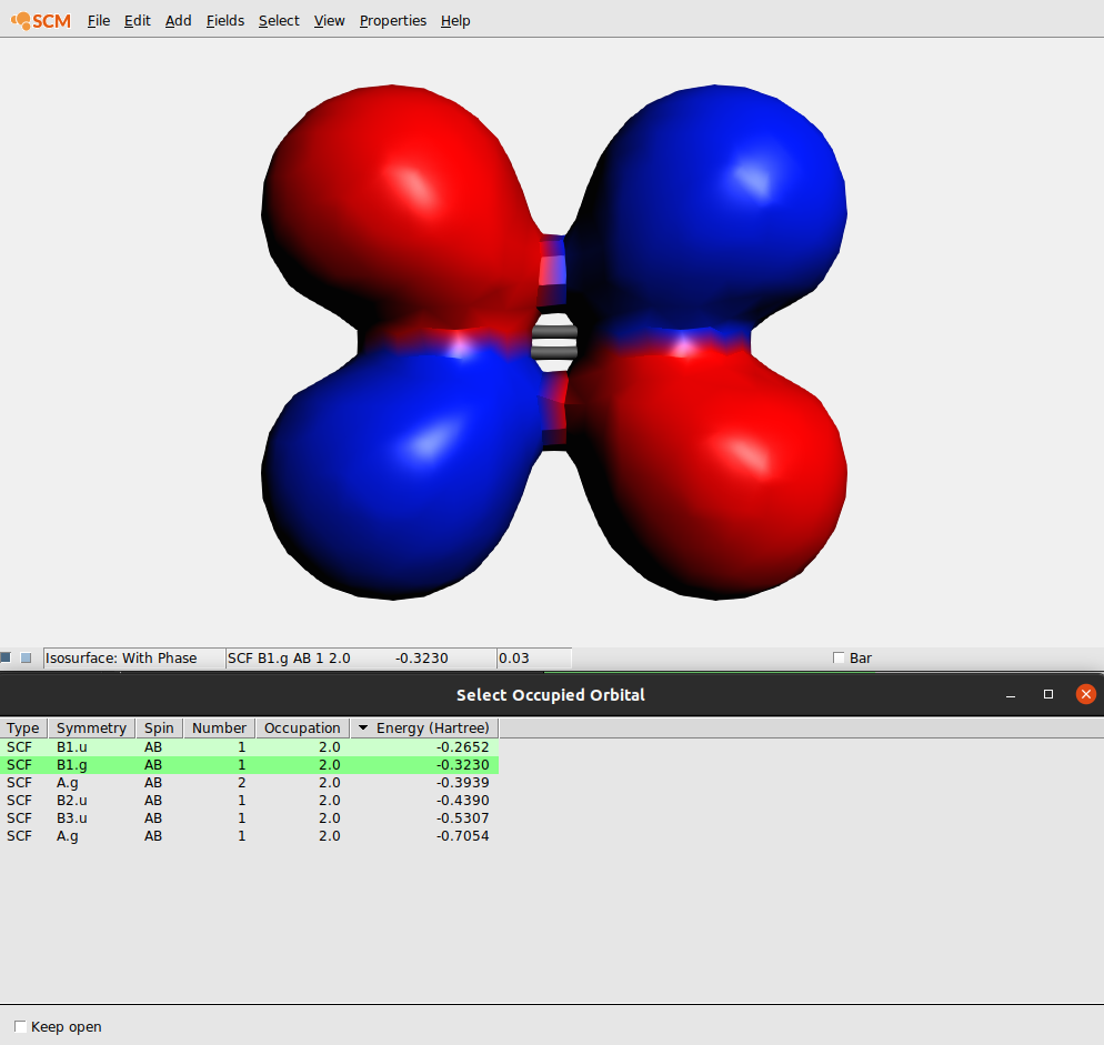
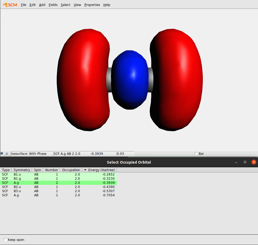
The Orbital select window allows you to reorder the orbitals by clicking on the headers of the columns. Thus you can sort by Symmetry, Spin, etc. Clicking again on a header reverts the sort order.
Transition density: AMSview
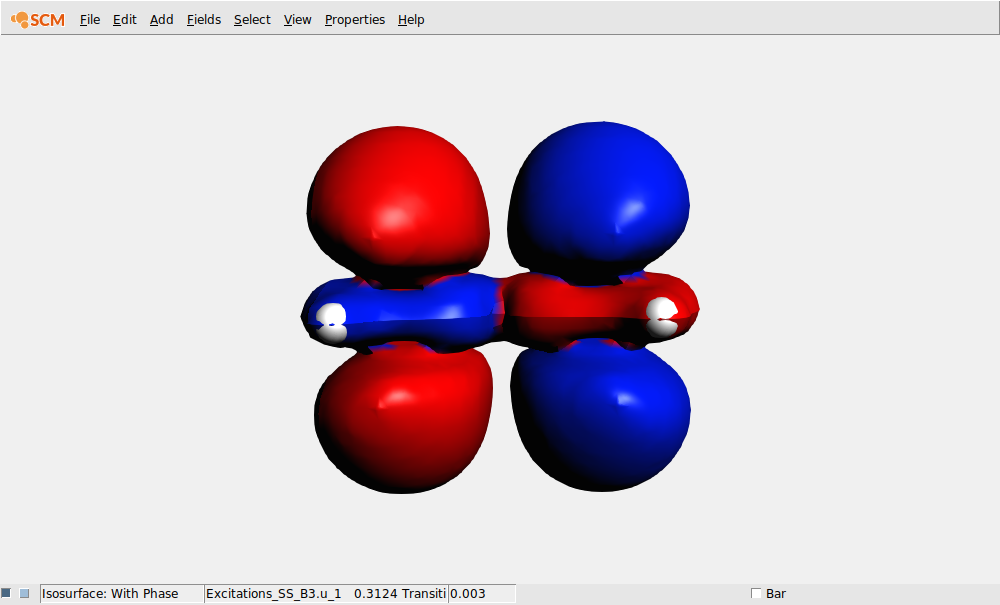
You can use AMSview to view orbitals etc, but also to have a look at the transition density.
In the field pull-down menu (in the control line for the isosurface with phase) you will find an entry ‘Transition (Fit) Density’, and if you select it an orbital select box will shown with all available transition densities:
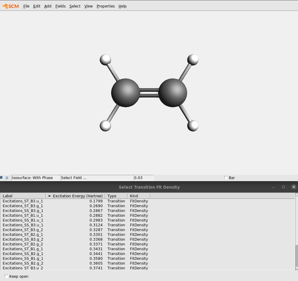
In this case lets select the transition density that belongs to the largest peak: the Singlet-Singlet excitation at 0.3123 Hartree (which may have B1.u, B2.u or B3.u symmetry depending on the molecule orientation):
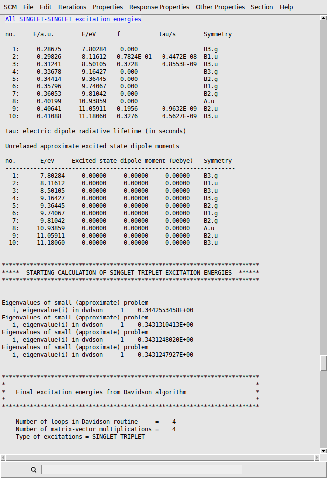
AMSoutput
Using the output browser you can find all details about your excitation calculation. Use the menu to jump to the relevant part of output:
KFBrowser: KF files, copy to Excel, graphs of results
Most result of the calculation are saved to the KF result file (the adf.rkf file for an ADF calculation). You can inspect the contents of KF files using the KFBrowser.
The KFBrowser gets the raw data out of the result file, and presents a selection of that might be of interest for users.
By default, KFBrowser opens the ams.rkf binary file. The ADF-specific results (such as excitations energies) are on the adf.rkf file.
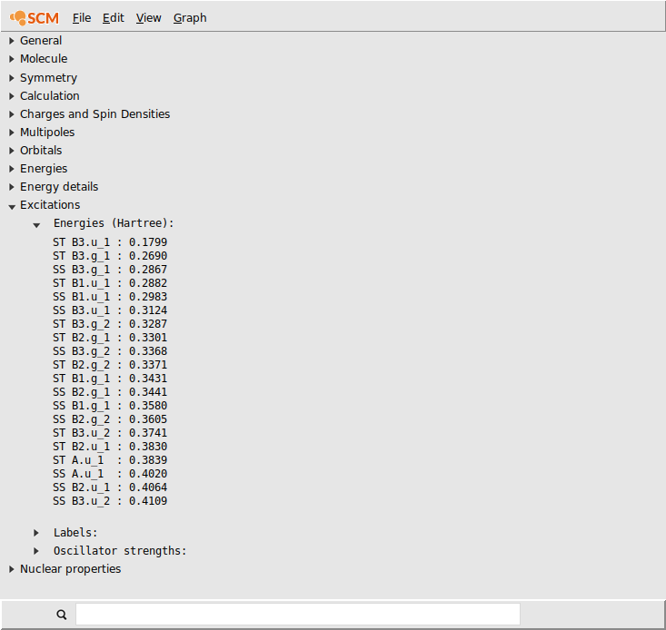
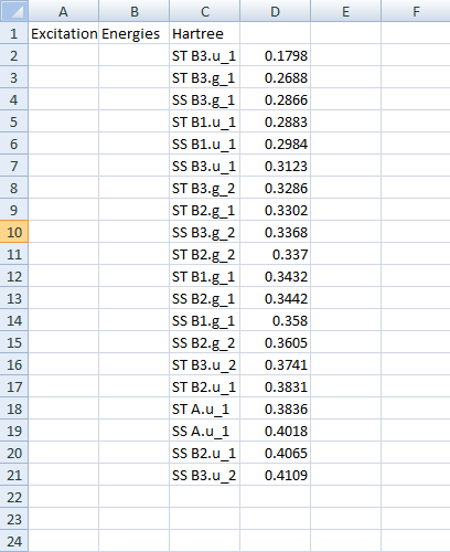
If you click on the name of the property you can select it. Next you can copy it, and paste it for example in Excel:
After pasting you should have your results nicely formatted in Excel or in some text document. Note that the values are tab-separated, so pasting into Excel will automatically put the data (energies) in cells.
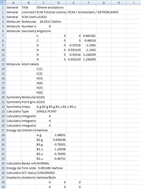
In a similar way you can copy/paste other results. Or even all results:
All results should be nicely formatted in your text document or spreadsheet:
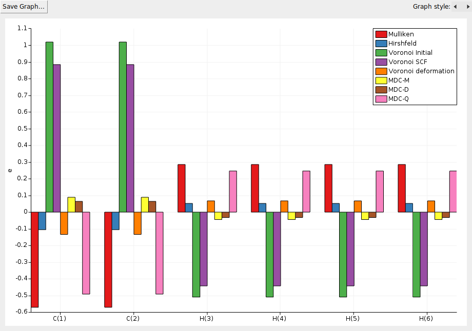
Another feature of the KFBrowser is that it can show results in simple graphs:
A window should appear that shows the selected results, charges in this case:
Finally two features that are intended for developers and expert users: the KFBrowser module can also show the raw data on the result file, and it can dump a KF file as a plain text file. To activate the expert mode, use the File → Expert Mode menu command. To save the contents of the result file as a text file using the File → Save As ASCII… command.
Excited state geometry optimization and excited state density
With ADF you can also optimize the geometry of some selected excited state. It depends on your application which state to optimize, in this tutorial we will pick the state corresponding to the largest peak in the UV/Vis spectrum.
AMSinput should open with the ethene-exci job (or come to the front if already open).
With AMSview you can see how the excited state geometry is different from the ground state geometry:
With AMSmovie you can see how the excited state density is different from the ground state density:
Now you see how the excited state density differs from the ground state density (for this geometry)
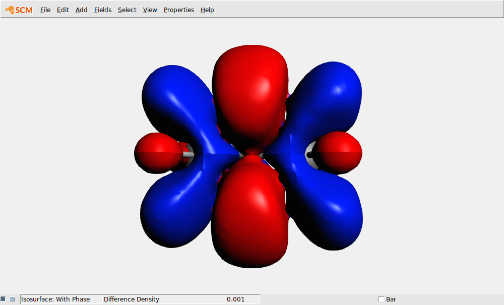
If you wish to see the excited state density, you can do this using a Calculated field (add the ground state density to the difference density).
Closing the AMS-GUI modules
To close only the current AMS-GUI module, use the Quit command from the SCM menu:
To close all AMS-GUI modules for your calculation at once, use the Close Job command from the File menu:
Close Job will close all open modules that have your current job loaded, except AMSjobs.
Finally, the Quit All command will close every AMS-GUI module, including AMSjobs:
All AMS-GUI modules will be closed.