Dihedral PES Scan with and without geometry optimization
This example runs a dihedral scan calculation as a PLAMS workflow and compares the two PES scan modes controlled by PESScan%Optimize. The notebook runs the same F-C-C-F dihedral scan twice: once as the default constrained optimization at each point, and once as a rigid scan without geometry optimization. It then overlays both potential energy curves and discusses the qualitative differences.
Overview
This notebook converts a shell-based AMS input for a dihedral scan into a PLAMS workflow. We will use the same molecule and the same F-C-C-F scan coordinate in two different PES scan modes:
PESScan%Optimize = "Yes": optimize all other degrees of freedom at every scanned dihedral.PESScan%Optimize = "No": perform a rigid scan and run only single-point calculations at the sampled geometries.
The goal is to compare the resulting potential energy curves and understand what changes when the rest of the molecule is allowed to relax.
Imports
import matplotlib.pyplot as plt
import numpy as np
from scm.base import ChemicalSystem
from scm.plams import AMSJob, Settings, Units, view
Units conversion
hartree_to_kcalmol = Units.convert(1.0, "hartree", "kcal/mol")
rad_to_deg = 180.0/np.pi
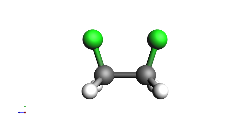
Starting structure
We start the chemical system using a System Block string. It’s important to note that we make initial guesses about the bonds. This is crucial for the setting PESScan%Optimize = "No" because rigid scans rely on the bond structure to determine which atoms will move when an internal coordinate changes.
system = ChemicalSystem(
"""
    System
        Atoms
            C 0.0 0.0 0.7613406700000001
            C 0.0 0.0 -0.7613406700000001
            H -0.8995903700000005 -0.4807776699999992 -1.16014003
            H 0.8995878199999997 -0.4807824600000009 -1.16014003
            F 3.450000001154741e-06 1.30012313 -1.17926967
            H 0.89958909 -0.48078006 1.16014003
            H -0.89958909 -0.48078006 1.16014003
            F 0.0 1.30012315 1.17926966
        End
    End
"""
)

system.guess_bonds()
view(system, direction="along_pca3")
Common PLAMS settings
The engine part of the original .run file is very small: it just uses the DFTB engine with default settings. We first create a Settings object with the common AMS and DFTB setup, and then copy it for the two scan modes.
common_settings = Settings()
common_settings.input.ams.Task = "PESScan"
common_settings.input.DFTB = Settings()

print(AMSJob(settings=common_settings, molecule=system, name="template").get_input())
Task PESScan

System
   Atoms
      C 0 0 0.7613406699999999
      C 0 0 -0.7613406699999999
      H -0.8995903700000005 -0.4807776699999992 -1.16014003
      H 0.8995878199999997 -0.4807824600000009 -1.16014003
      F 3.450000001154741e-06 1.30012313 -1.17926967
      H 0.89958909 -0.48078006 1.16014003
      H -0.89958909 -0.48078006 1.16014003
      F 0 1.30012315 1.17926966
   End
   BondOrders
      1 2 1
      1 6 1
      1 7 1
      1 8 1
      2 3 1
      2 4 1
      2 5 1
   End
End

Engine DFTB
EndEngine
Add the PES scan block
The original text input scans the dihedral defined by atoms 8 1 2 5 from 0 to 360 degrees using 41 points. In PLAMS, the same input is expressed through nested Settings keys. The only difference between the two settings objects below is the value of PESScan.Optimize.
settings_optimize_yes = common_settings.copy()
settings_optimize_yes.input.ams.PESScan.Optimize = "Yes"
settings_optimize_yes.input.ams.PESScan.ScanCoordinate.nPoints = 41
settings_optimize_yes.input.ams.PESScan.ScanCoordinate.Dihedral = "8 1 2 5 0 360"

settings_optimize_no = common_settings.copy()
settings_optimize_no.input.ams.PESScan.Optimize = "No"
settings_optimize_no.input.ams.PESScan.ScanCoordinate.nPoints = 41
settings_optimize_no.input.ams.PESScan.ScanCoordinate.Dihedral = "8 1 2 5 0 360"
Create and run the two jobs
We now create the two jobs directly from the two settings objects. Running both jobs gives us two PES curves that differ only by the treatment of the remaining degrees of freedom.
job_optimize_yes = AMSJob(
    molecule=system.copy(),
    settings=settings_optimize_yes,
    name="dihedral_scan_optimize_yes",
)
job_optimize_no = AMSJob(
    molecule=system.copy(),
    settings=settings_optimize_no,
    name="dihedral_scan_optimize_no",
)

job_optimize_yes.run();
job_optimize_no.run();
[10.06|11:46:14] JOB dihedral_scan_optimize_yes STARTED
[10.06|11:46:14] JOB dihedral_scan_optimize_yes RUNNING
[10.06|11:46:18] JOB dihedral_scan_optimize_yes FINISHED
[10.06|11:46:18] JOB dihedral_scan_optimize_yes SUCCESSFUL
[10.06|11:46:18] JOB dihedral_scan_optimize_no STARTED
[10.06|11:46:18] JOB dihedral_scan_optimize_no RUNNING
[10.06|11:46:19] JOB dihedral_scan_optimize_no FINISHED
[10.06|11:46:19] JOB dihedral_scan_optimize_no SUCCESSFUL
Extract the scan coordinates and relative energies
AMS stores PES scan data in the PESScan section of the results file. The get_pesscan_results() method returns the scanned coordinates and the energies in a convenient dictionary.
results_optimize_yes = job_optimize_yes.results.get_pesscan_results()
dihedrals_optimize_yes = np.array(results_optimize_yes["RaveledPESCoords"][0]) * rad_to_deg
energies_optimize_yes = np.array(results_optimize_yes["PES"]) * hartree_to_kcalmol
relative_energies_optimize_yes = energies_optimize_yes - min(energies_optimize_yes)
results_optimize_no = job_optimize_no.results.get_pesscan_results()
dihedrals_optimize_no = np.array(results_optimize_no["RaveledPESCoords"][0]) * rad_to_deg
energies_optimize_no = np.array(results_optimize_no["PES"]) * hartree_to_kcalmol
relative_energies_optimize_no = energies_optimize_no - min(energies_optimize_no)
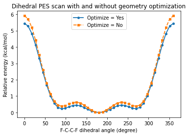
print(f"Optimize = Yes: maximum relative energy = {max(relative_energies_optimize_yes):.2f} kcal/mol")
print(f"Optimize = No: maximum relative energy = {max(relative_energies_optimize_no):.2f} kcal/mol")
Optimize = Yes: maximum relative energy = 5.44 kcal/mol
Optimize = No: maximum relative energy = 5.91 kcal/mol
Plot the potential energy curves
fig, ax = plt.subplots()
ax.plot(
    dihedrals_optimize_yes,
    relative_energies_optimize_yes,
    marker="o",
    linestyle="-",
    color="tab:blue",
    linewidth=1.8,
    markersize=4,
    label="Optimize = Yes",
)
ax.plot(
    dihedrals_optimize_no,
    relative_energies_optimize_no,
    marker="s",
    linestyle="--",
    color="tab:orange",
    linewidth=1.8,
    markersize=4,
    label="Optimize = No",
)
ax.set_xlabel("F-C-C-F dihedral angle (degree)")
ax.set_ylabel("Relative energy (kcal/mol)")
ax.legend()
ax;
Discussion
When PESScan%Optimize = "Yes", every sampled dihedral is treated as a constrained geometry optimization. The scanned F-C-C-F angle is fixed, but the rest of the molecule can relax. This usually lowers the energy at each point and often smooths the curve.
When PESScan%Optimize = "No", AMS directly changes the dihedral and evaluates the energy of that geometry without any further relaxation. This rigid scan is cheaper and can be useful for fast exploration, but it generally keeps more strain in the structure.
After running the notebook, compare the barrier heights and the detailed shape of the two curves. The rigid scan is expected to sit higher in energy at many points, because nearby bond lengths and angles are not allowed to adapt to the imposed dihedral.
See also
Python Script
#!/usr/bin/env python
# coding: utf-8

# ## Overview
#
# This notebook converts a shell-based AMS input for a dihedral scan into a PLAMS workflow.
# We will use the same molecule and the same F-C-C-F scan coordinate in two different PES scan modes:
#
# - `PESScan%Optimize = "Yes"`: optimize all other degrees of freedom at every scanned dihedral.
# - `PESScan%Optimize = "No"`: perform a rigid scan and run only single-point calculations at the sampled geometries.
#
# The goal is to compare the resulting potential energy curves and understand what changes when the rest of the molecule is allowed to relax.

# ## Imports

import matplotlib.pyplot as plt
import numpy as np
from scm.base import ChemicalSystem
from scm.plams import AMSJob, Settings, Units, view


# ## Units conversion

hartree_to_kcalmol = Units.convert(1.0, "hartree", "kcal/mol")
rad_to_deg = 180.0/np.pi


# ## Starting structure
#
# We start the chemical system using a `System Block` string. It's important to note that we make initial guesses about the bonds. This is crucial for the setting `PESScan%Optimize = "No"` because rigid scans rely on the bond structure to determine which atoms will move when an internal coordinate changes.

system = ChemicalSystem(
"""
    System
        Atoms
            C 0.0 0.0 0.7613406700000001
            C 0.0 0.0 -0.7613406700000001
            H -0.8995903700000005 -0.4807776699999992 -1.16014003
            H 0.8995878199999997 -0.4807824600000009 -1.16014003
            F 3.450000001154741e-06 1.30012313 -1.17926967
            H 0.89958909 -0.48078006 1.16014003
            H -0.89958909 -0.48078006 1.16014003
            F 0.0 1.30012315 1.17926966
        End
    End
"""
)

system.guess_bonds()
view(system, direction="along_pca3", picture_path="picture1.png")


# ## Common PLAMS settings
#
# The engine part of the original `.run` file is very small: it just uses the DFTB engine with default settings. We first create a `Settings` object with the common AMS and DFTB setup, and then copy it for the two scan modes.

common_settings = Settings()
common_settings.input.ams.Task = "PESScan"
common_settings.input.DFTB = Settings()

print(AMSJob(settings=common_settings, molecule=system, name="template").get_input())


# ## Add the PES scan block
#
# The original text input scans the dihedral defined by atoms `8 1 2 5` from `0` to `360` degrees using `41` points.
# In PLAMS, the same input is expressed through nested `Settings` keys. The only difference between the two settings objects below is the value of `PESScan.Optimize`.

settings_optimize_yes = common_settings.copy()
settings_optimize_yes.input.ams.PESScan.Optimize = "Yes"
settings_optimize_yes.input.ams.PESScan.ScanCoordinate.nPoints = 41
settings_optimize_yes.input.ams.PESScan.ScanCoordinate.Dihedral = "8 1 2 5 0 360"

settings_optimize_no = common_settings.copy()
settings_optimize_no.input.ams.PESScan.Optimize = "No"
settings_optimize_no.input.ams.PESScan.ScanCoordinate.nPoints = 41
settings_optimize_no.input.ams.PESScan.ScanCoordinate.Dihedral = "8 1 2 5 0 360"


# ## Create and run the two jobs
#
# We now create the two jobs directly from the two settings objects. Running both jobs gives us two PES curves that differ only by the treatment of the remaining degrees of freedom.

job_optimize_yes = AMSJob(
    molecule=system.copy(),
    settings=settings_optimize_yes,
    name="dihedral_scan_optimize_yes",
)
job_optimize_no = AMSJob(
    molecule=system.copy(),
    settings=settings_optimize_no,
    name="dihedral_scan_optimize_no",
)

job_optimize_yes.run();
job_optimize_no.run();


# ## Extract the scan coordinates and relative energies
#
# AMS stores PES scan data in the `PESScan` section of the results file. The `get_pesscan_results()` method returns the scanned coordinates and the energies in a convenient dictionary.

results_optimize_yes = job_optimize_yes.results.get_pesscan_results()
dihedrals_optimize_yes = np.array(results_optimize_yes["RaveledPESCoords"][0]) * rad_to_deg
energies_optimize_yes = np.array(results_optimize_yes["PES"]) * hartree_to_kcalmol
relative_energies_optimize_yes = energies_optimize_yes - min(energies_optimize_yes)

results_optimize_no = job_optimize_no.results.get_pesscan_results()
dihedrals_optimize_no = np.array(results_optimize_no["RaveledPESCoords"][0]) * rad_to_deg
energies_optimize_no = np.array(results_optimize_no["PES"]) * hartree_to_kcalmol
relative_energies_optimize_no = energies_optimize_no - min(energies_optimize_no)

print(f"Optimize = Yes: maximum relative energy = {max(relative_energies_optimize_yes):.2f} kcal/mol")
print(f"Optimize = No: maximum relative energy = {max(relative_energies_optimize_no):.2f} kcal/mol")


# ## Plot the potential energy curves

fig, ax = plt.subplots()
ax.plot(
    dihedrals_optimize_yes,
    relative_energies_optimize_yes,
    marker="o",
    linestyle="-",
    color="tab:blue",
    linewidth=1.8,
    markersize=4,
    label="Optimize = Yes",
)
ax.plot(
    dihedrals_optimize_no,
    relative_energies_optimize_no,
    marker="s",
    linestyle="--",
    color="tab:orange",
    linewidth=1.8,
    markersize=4,
    label="Optimize = No",
)
ax.set_xlabel("F-C-C-F dihedral angle (degree)")
ax.set_ylabel("Relative energy (kcal/mol)")
ax.legend()
ax;
ax.figure.savefig("picture2.png")


# ## Discussion
#
# When `PESScan%Optimize = "Yes"`, every sampled dihedral is treated as a constrained geometry optimization. The scanned F-C-C-F angle is fixed, but the rest of the molecule can relax. This usually lowers the energy at each point and often smooths the curve.
#
# When `PESScan%Optimize = "No"`, AMS directly changes the dihedral and evaluates the energy of that geometry without any further relaxation. This rigid scan is cheaper and can be useful for fast exploration, but it generally keeps more strain in the structure.
#
# After running the notebook, compare the barrier heights and the detailed shape of the two curves. The rigid scan is expected to sit higher in energy at many points, because nearby bond lengths and angles are not allowed to adapt to the imposed dihedral.