Transition state - Polymerization catalyst¶

Downloads: Notebook | Script ?

Estimated time: 0.50 hours

Requires: AMS2026 or later

GUI tutorial: Ziegler-Natta Catalyst

../_images/transition_state_polymerization_catalyst_16_1.png

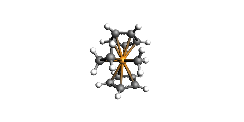
Optimized transition state.

../_images/transition_state_polymerization_catalyst_13_0.png — Results from PES Scan (maximum energy for approximate transition state structure).¶

Plan¶

This tutorial shows how to

optimize the reactant state,
perform a PES Scan to get a good starting structure for transition state search,
perform a transition state search,
extract the barrier

Note that this tutorial only shows one half of a reaction.

Initial imports¶

from scm.base import ChemicalSystem
from scm.plams import view, Settings, AMSJob, Units

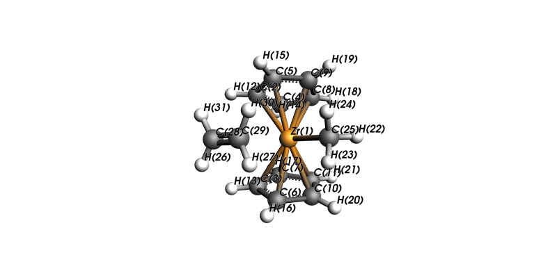
Initial system¶

mol = ChemicalSystem(
    """
System
    Charge 1.0
    Atoms
        Zr       1.60682759      -9.09697636       1.29667400
        C       2.89496678     -10.06750666       3.11673910
        C       2.84805610      -9.90469975      -0.63831357
        C       1.91952398     -11.03393562       2.76898899
        C       2.21720521      -8.93716871       3.64709384
        C       2.05919385      -8.80831375      -1.07706558
        C       1.96898612     -10.95146163      -0.26897070
        C       0.63990901     -10.49043590       3.04466191
        C       0.82713373      -9.20286661       3.61113029
        C       0.69607878      -9.17611676      -0.96529901
        C       0.63812917     -10.49403820      -0.44270184
        H       3.96827494     -10.23973626       3.15013890
        H       3.92582990      -9.99794535      -0.74784951
        H       2.12190386     -12.06174102       2.48123664
        H       2.68569500      -8.09238646       4.14547290
        H       2.43329579      -7.91168000      -1.56456659
        H       2.26368032     -11.97103749      -0.03692581
        H      -0.30289388     -11.03081473       2.99676260
        H       0.05404650      -8.59747583       4.07520644
        H      -0.14620660      -8.61151792      -1.35464113
        H      -0.25838864     -11.10457655      -0.36003217
        H      -0.85662057      -7.76723654       1.38227139
        H       0.26321351      -6.74399730       0.47215750
        H       0.31659006      -6.75672110       2.23713123
        C       0.17801499      -7.39347280       1.35339060
        H       4.83158681      -7.79302616       0.33628574
        H       2.98632816      -6.14645123       0.41958259
        C       4.37932750      -7.48955975       1.27484960
        C       3.37901781      -6.61143075       1.32052856
        H       3.01865674      -6.20459134       2.26225286
        H       4.86414560      -7.85327440       2.17514370
    End
End"""
)
mol.guess_bonds()
print(f"{mol.charge=}")
view(mol, direction="along_y", show_atom_labels=True, atom_label_type="Name")

mol.charge=1.0

../_images/transition_state_polymerization_catalyst_4_1.png

DFTB Settings¶

from scm.plams import Settings, AMSJob


def get_dftb_settings():
    # Engine settings: GFN-1xTB with implicit Tolene solvation
    settings = Settings()
    settings.input.DFTB.Model = "GFN1-xTB"
    settings.input.DFTB.Solvation.Solvent = "Toluene"
    return settings


print(AMSJob(settings=get_dftb_settings()).get_input())

Engine DFTB
  Model GFN1-xTB
  Solvation
    Solvent Toluene
  End
EndEngine

Geometry optimization of reactant state¶

def get_reactants_job(mol):
    settings = get_dftb_settings()
    settings.input.ams.Task = "SinglePoint"
    settings.input.ams.Properties.NormalModes = "Yes"
    job = AMSJob(molecule=mol, settings=settings, name="reactants_frequencies")
    return job


reactants_job = get_reactants_job(mol)
reactants_job.run();

[16.12|15:06:37] JOB reactants_frequencies STARTED
[16.12|15:06:37] JOB reactants_frequencies RUNNING
[16.12|15:06:40] JOB reactants_frequencies FINISHED
[16.12|15:06:40] JOB reactants_frequencies SUCCESSFUL

Set up PES Scan to find approximate transition state¶

def get_pesscan_job(mol):
    # Engine settings: GFN-1xTB with implicit Tolene solvation
    settings = get_dftb_settings()

    # AMS settings for PES scan (see online tutorial for choice of scan coordinates)
    settings.input.ams.Task = "PESScan"
    settings.input.ams.PESScan.ScanCoordinate.nPoints = "20"
    settings.input.ams.PESScan.ScanCoordinate.Distance = ["1 28 3.205 2.3", "29 25 3.295 1.5"]

    # Loosened convergence criteria
    settings.input.ams.GeometryOptimization.Convergence.Energy = "5.0e-5 [Hartree]"
    settings.input.ams.GeometryOptimization.Convergence.Gradients = "5.0e-3"
    settings.input.ams.GeometryOptimization.Convergence.Step = "5.0e-3 [Angstrom]"

    # setting up the AMS job with the molecule and settings object
    job = AMSJob(molecule=mol, settings=settings, name="pes_scan")
    return job

    # run the calulation


pesscan_job = get_pesscan_job(reactants_job.results.get_main_system())
pesscan_job.run();

[16.12|15:06:40] JOB pes_scan STARTED
[16.12|15:06:40] JOB pes_scan RUNNING
[16.12|15:07:13] JOB pes_scan FINISHED
[16.12|15:07:13] JOB pes_scan SUCCESSFUL

PESScan results¶

import matplotlib.pyplot as plt
from pprint import pprint

pesscan_results = pesscan_job.results.get_pesscan_results()
pprint(pesscan_results, depth=1)

{'ConstrainedAtoms': {1, 28, 29, 25},
 'Converged': [...],
 'HistoryIndices': [...],
 'Molecules': [...],
 'OrigScanCoords': [...],
 'PES': [...],
 'Properties': [],
 'RaveledPESCoords': [...],
 'RaveledScanCoords': [...],
 'RaveledUnits': [...],
 'ScanCoords': [...],
 'Units': [...],
 'nPESPoints': 20,
 'nRaveledScanCoords': 2,
 'nScanCoords': 1}

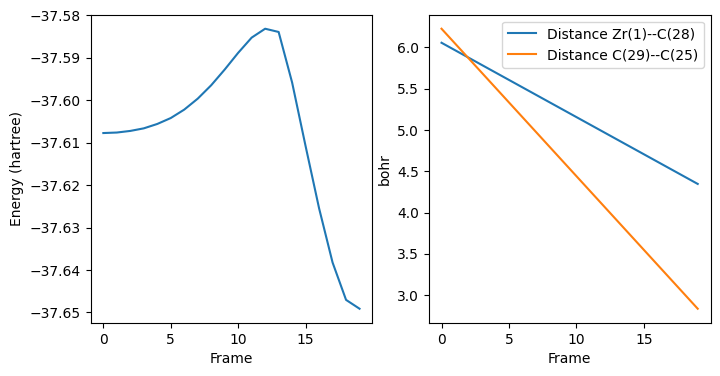
fix, ax = plt.subplots(1, 2, figsize=(8, 4))
ax[0].plot(list(range(pesscan_results["nPESPoints"])), pesscan_results["PES"])
ax[0].set_ylabel("Energy (hartree)")
ax[0].set_xlabel("Frame")
for i in range(pesscan_results["nRaveledScanCoords"]):
    ax[1].plot(
        list(range(pesscan_results["nPESPoints"])),
        pesscan_results["RaveledPESCoords"][i],
        label=pesscan_results["RaveledScanCoords"][i],
    )
ax[1].set_ylabel("bohr")
ax[1].set_xlabel("Frame")
ax[1].legend();

import numpy as np

highest_energy = np.max(pesscan_results["PES"])
highest_energy_index = np.argmax(pesscan_results["PES"])

# res['Molecules'] contains all the converged geometries (as PLAMS Molecules)
highest_energy_geo = pesscan_results["Molecules"][highest_energy_index]

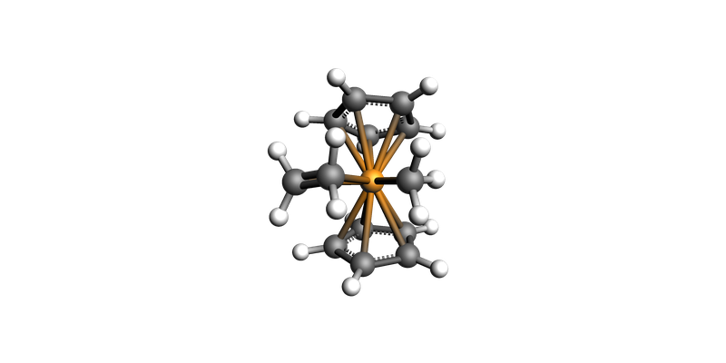
print(f"Highest energy: {highest_energy:.6f} hartree, for geometry #{highest_energy_index+1}")
print("We will use that structure as starting point for TS search")
highest_energy_geo.guess_bonds()
view(highest_energy_geo, direction="along_y")

Highest energy: -37.583147 hartree, for geometry #13
We will use that structure as starting point for TS search

../_images/transition_state_polymerization_catalyst_14_1.png

Transition state search¶

def get_ts_job(mol):
    settings = get_dftb_settings()

    # AMS settings for TS search
    settings.input.ams.Task = "TransitionStateSearch"
    settings.input.ams.Properties.NormalModes = "Yes"
    settings.input.ams.GeometryOptimization.InitialHessian.Type = "Calculate"

    # setting up the AMS job with the molecule and settings object
    job = AMSJob(molecule=mol, settings=settings, name="ts_search")
    return job


ts_job = get_ts_job(highest_energy_geo)
ts_job.run()
ts_mol = ts_job.results.get_main_system()
ts_mol.guess_bonds()
view(ts_mol, direction="along_y")

[16.12|15:07:15] JOB ts_search STARTED
[16.12|15:07:15] JOB ts_search RUNNING
[16.12|15:07:26] JOB ts_search FINISHED
[16.12|15:07:26] JOB ts_search SUCCESSFUL

def get_gibbs_energy(job: AMSJob, unit="hartree"):
    gibbs_energy = job.results.readrkf("Thermodynamics", "Gibbs free Energy", file="engine")
    gibbs_energy *= Units.convert(1.0, "hartree", unit)
    return gibbs_energy


def print_ts_results(job):
    energy = job.results.get_energy(unit="kcal/mol")
    gibbs_energy = get_gibbs_energy(job, unit="kcal/mol")
    frequencies = job.results.get_frequencies(unit="cm^-1")
    character = job.results.readrkf("AMSResults", "PESPointCharacter", file="engine")

    # print results
    print("== Results ==")
    print("Character   : {}".format(character))
    print("Energy      : {:.3f} kcal/mol".format(energy))
    print("Gibbs Energy: {:.3f} kcal/mol".format(gibbs_energy))
    for freq in frequencies:
        if freq < 0:
            print("Imaginary frequency : {:.3f} cm^-1".format(freq))
        else:
            break


print_ts_results(ts_job)

== Results ==
Character   : transition state
Energy      : -23587.067 kcal/mol
Gibbs Energy: -23460.913 kcal/mol
Imaginary frequency : -397.387 cm^-1

Free energy barrier¶

def print_final_results(gibbs_energy_ts: float, gibbs_energy_reactants: float, T=298.15):
    barrier = gibbs_energy_ts - gibbs_energy_reactants  # kJ/mol
    NA = 6.022e23  # Avogadro's constant
    k_B = 1.380649e-23  # Boltzmann constant, J / (mol*K)
    h = 6.626e-34  # Planck's constant, J * s
    rate_constant = (k_B * T / h) * np.exp(-barrier * 1000 / (NA * k_B * T))
    print("Results summary")
    print("Reactants Gibbs Energy: {:.3f} kJ/mol".format(gibbs_energy_reactants))
    print("TS Gibbs Energy:        {:.3f} kJ/mol".format(gibbs_energy_ts))
    print("Free energy barrier:    {:.3f} kJ/mol".format(barrier))
    print("Rate constant:          {:.3f} s⁻¹ at {} K".format(rate_constant, T))


gibbs_energy_ts = get_gibbs_energy(ts_job, "kJ/mol")
gibbs_energy_reactants = get_gibbs_energy(reactants_job, "kJ/mol")
print_final_results(gibbs_energy_ts, gibbs_energy_reactants, T=298.15)

Results summary
Reactants Gibbs Energy: -98216.185 kJ/mol
TS Gibbs Energy:        -98160.461 kJ/mol
Free energy barrier:    55.724 kJ/mol
Rate constant:          1073.251 s⁻¹ at 298.15 K

Python Script¶

#!/usr/bin/env python
# coding: utf-8

# ## Plan
#
# This tutorial shows how to
#
# * optimize the reactant state,
# * perform a PES Scan to get a good starting structure for transition state search,
# * perform a transition state search,
# * extract the barrier
#
# Note that this tutorial only shows one half of a reaction.

# ## Initial imports

from scm.base import ChemicalSystem
from scm.plams import view, Settings, AMSJob, Units


# ## Initial system

mol = ChemicalSystem(
    """
System
    Charge 1.0
    Atoms
        Zr       1.60682759      -9.09697636       1.29667400
        C       2.89496678     -10.06750666       3.11673910
        C       2.84805610      -9.90469975      -0.63831357
        C       1.91952398     -11.03393562       2.76898899
        C       2.21720521      -8.93716871       3.64709384
        C       2.05919385      -8.80831375      -1.07706558
        C       1.96898612     -10.95146163      -0.26897070
        C       0.63990901     -10.49043590       3.04466191
        C       0.82713373      -9.20286661       3.61113029
        C       0.69607878      -9.17611676      -0.96529901
        C       0.63812917     -10.49403820      -0.44270184
        H       3.96827494     -10.23973626       3.15013890
        H       3.92582990      -9.99794535      -0.74784951
        H       2.12190386     -12.06174102       2.48123664
        H       2.68569500      -8.09238646       4.14547290
        H       2.43329579      -7.91168000      -1.56456659
        H       2.26368032     -11.97103749      -0.03692581
        H      -0.30289388     -11.03081473       2.99676260
        H       0.05404650      -8.59747583       4.07520644
        H      -0.14620660      -8.61151792      -1.35464113
        H      -0.25838864     -11.10457655      -0.36003217
        H      -0.85662057      -7.76723654       1.38227139
        H       0.26321351      -6.74399730       0.47215750
        H       0.31659006      -6.75672110       2.23713123
        C       0.17801499      -7.39347280       1.35339060
        H       4.83158681      -7.79302616       0.33628574
        H       2.98632816      -6.14645123       0.41958259
        C       4.37932750      -7.48955975       1.27484960
        C       3.37901781      -6.61143075       1.32052856
        H       3.01865674      -6.20459134       2.26225286
        H       4.86414560      -7.85327440       2.17514370
    End
End"""
)
mol.guess_bonds()
print(f"{mol.charge=}")
view(mol, direction="along_y", show_atom_labels=True, atom_label_type="Name", picture_path="picture1.png")


# ## DFTB Settings

from scm.plams import Settings, AMSJob


def get_dftb_settings():
    # Engine settings: GFN-1xTB with implicit Tolene solvation
    settings = Settings()
    settings.input.DFTB.Model = "GFN1-xTB"
    settings.input.DFTB.Solvation.Solvent = "Toluene"
    return settings


print(AMSJob(settings=get_dftb_settings()).get_input())


# ## Geometry optimization of reactant state


def get_reactants_job(mol):
    settings = get_dftb_settings()
    settings.input.ams.Task = "SinglePoint"
    settings.input.ams.Properties.NormalModes = "Yes"
    job = AMSJob(molecule=mol, settings=settings, name="reactants_frequencies")
    return job


reactants_job = get_reactants_job(mol)
reactants_job.run()


# ## Set up PES Scan to find approximate transition state


def get_pesscan_job(mol):
    # Engine settings: GFN-1xTB with implicit Tolene solvation
    settings = get_dftb_settings()

    # AMS settings for PES scan (see online tutorial for choice of scan coordinates)
    settings.input.ams.Task = "PESScan"
    settings.input.ams.PESScan.ScanCoordinate.nPoints = "20"
    settings.input.ams.PESScan.ScanCoordinate.Distance = ["1 28 3.205 2.3", "29 25 3.295 1.5"]

    # Loosened convergence criteria
    settings.input.ams.GeometryOptimization.Convergence.Energy = "5.0e-5 [Hartree]"
    settings.input.ams.GeometryOptimization.Convergence.Gradients = "5.0e-3"
    settings.input.ams.GeometryOptimization.Convergence.Step = "5.0e-3 [Angstrom]"

    # setting up the AMS job with the molecule and settings object
    job = AMSJob(molecule=mol, settings=settings, name="pes_scan")
    return job

    # run the calulation


pesscan_job = get_pesscan_job(reactants_job.results.get_main_system())
pesscan_job.run()


# ## PESScan results

import matplotlib.pyplot as plt
from pprint import pprint

pesscan_results = pesscan_job.results.get_pesscan_results()
pprint(pesscan_results, depth=1)


fix, ax = plt.subplots(1, 2, figsize=(8, 4))
ax[0].plot(list(range(pesscan_results["nPESPoints"])), pesscan_results["PES"])
ax[0].set_ylabel("Energy (hartree)")
ax[0].set_xlabel("Frame")
for i in range(pesscan_results["nRaveledScanCoords"]):
    ax[1].plot(
        list(range(pesscan_results["nPESPoints"])),
        pesscan_results["RaveledPESCoords"][i],
        label=pesscan_results["RaveledScanCoords"][i],
    )
ax[1].set_ylabel("bohr")
ax[1].set_xlabel("Frame")
ax[1].legend()


import numpy as np

highest_energy = np.max(pesscan_results["PES"])
highest_energy_index = np.argmax(pesscan_results["PES"])

# res['Molecules'] contains all the converged geometries (as PLAMS Molecules)
highest_energy_geo = pesscan_results["Molecules"][highest_energy_index]

print(f"Highest energy: {highest_energy:.6f} hartree, for geometry #{highest_energy_index+1}")
print("We will use that structure as starting point for TS search")
highest_energy_geo.guess_bonds()
view(highest_energy_geo, direction="along_y", picture_path="picture2.png")


# ## Transition state search


def get_ts_job(mol):
    settings = get_dftb_settings()

    # AMS settings for TS search
    settings.input.ams.Task = "TransitionStateSearch"
    settings.input.ams.Properties.NormalModes = "Yes"
    settings.input.ams.GeometryOptimization.InitialHessian.Type = "Calculate"

    # setting up the AMS job with the molecule and settings object
    job = AMSJob(molecule=mol, settings=settings, name="ts_search")
    return job


ts_job = get_ts_job(highest_energy_geo)
ts_job.run()
ts_mol = ts_job.results.get_main_system()
ts_mol.guess_bonds()
view(ts_mol, direction="along_y", picture_path="picture3.png")


def get_gibbs_energy(job: AMSJob, unit="hartree"):
    gibbs_energy = job.results.readrkf("Thermodynamics", "Gibbs free Energy", file="engine")
    gibbs_energy *= Units.convert(1.0, "hartree", unit)
    return gibbs_energy


def print_ts_results(job):
    energy = job.results.get_energy(unit="kcal/mol")
    gibbs_energy = get_gibbs_energy(job, unit="kcal/mol")
    frequencies = job.results.get_frequencies(unit="cm^-1")
    character = job.results.readrkf("AMSResults", "PESPointCharacter", file="engine")

    # print results
    print("== Results ==")
    print("Character   : {}".format(character))
    print("Energy      : {:.3f} kcal/mol".format(energy))
    print("Gibbs Energy: {:.3f} kcal/mol".format(gibbs_energy))
    for freq in frequencies:
        if freq < 0:
            print("Imaginary frequency : {:.3f} cm^-1".format(freq))
        else:
            break


print_ts_results(ts_job)


# ## Free energy barrier


def print_final_results(gibbs_energy_ts: float, gibbs_energy_reactants: float, T=298.15):
    barrier = gibbs_energy_ts - gibbs_energy_reactants  # kJ/mol
    NA = 6.022e23  # Avogadro's constant
    k_B = 1.380649e-23  # Boltzmann constant, J / (mol*K)
    h = 6.626e-34  # Planck's constant, J * s
    rate_constant = (k_B * T / h) * np.exp(-barrier * 1000 / (NA * k_B * T))
    print("Results summary")
    print("Reactants Gibbs Energy: {:.3f} kJ/mol".format(gibbs_energy_reactants))
    print("TS Gibbs Energy:        {:.3f} kJ/mol".format(gibbs_energy_ts))
    print("Free energy barrier:    {:.3f} kJ/mol".format(barrier))
    print("Rate constant:          {:.3f} s⁻¹ at {} K".format(rate_constant, T))


gibbs_energy_ts = get_gibbs_energy(ts_job, "kJ/mol")
gibbs_energy_reactants = get_gibbs_energy(reactants_job, "kJ/mol")
print_final_results(gibbs_energy_ts, gibbs_energy_reactants, T=298.15)

Transition state - Polymerization catalyst¶

Plan¶

Initial imports¶

Initial system¶

DFTB Settings¶

Geometry optimization of reactant state¶

Set up PES Scan to find approximate transition state¶

PESScan results¶

Transition state search¶

Free energy barrier¶

Python Script¶

Related Documentation¶