COSMO-RS with multi-species components

Sometimes molecules behave in solution in ways that are not accurately captured by the “one-molecule-one-structure” paradigm of standard COSMO-RS theory. The single-structure picture of standard COSMO-RS represents much of the chemical space reasonably well but often fails to accurately describe solutions with more complex behavior. Examples of systems with complex behavior may include:

• Compounds that exist as multiple conformers

• Compounds that may dimerize, trimerize, etc.

• Compounds that can dissociate into multiple species

• Compounds or species that explicitly associate with other molecules (e.g., solvent) in solution

Multi-species COSMO-RS aims to describe the inherent complexities in these types of systems by allowing users to directly input multiple representations for a single component. The ratios of all of these species in solution are calculated and final, “apparent” values are reported for important thermodynamic values with respect to the compounds.

The following tutorial aims to guide the user in setting up and running calculations containing multi-species compounds. This guide will also discuss a few tips and point to a few GUI features that may be useful in understanding the results of the multi-species calculations. Additionally, we will walk the user through a number of practical examples demonstrating the benefits of this approach.

Building multi-species compounds

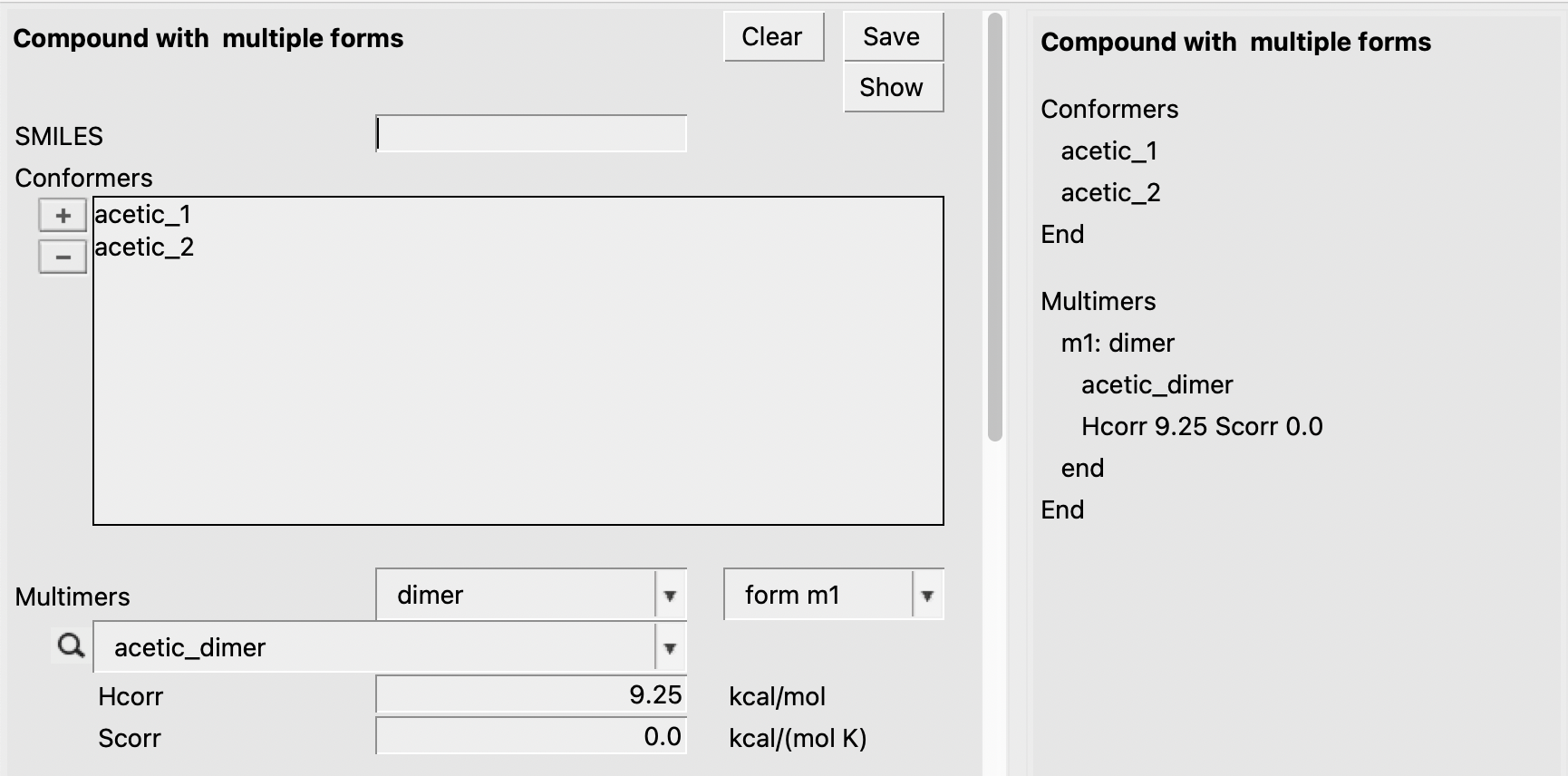
The multi-species compounds input is used to organize information about a compound that can exist in multiple forms. It can be accessed in the COSMO-RS GUI with a single step:

In this window, we can input .coskf files in specific boxes which convey a relationship between a .coskf file and a single molecule of the parent compound or a molecule which must be present for an associated form to occur. .coskf files can be used directly from the AMS sigma profile database or calculated with ADF by following this tutorial. A basic guide for inputting .multipleform compounds is given below:

Select Compounds → Compound with multiple forms

Input all conformers under conformers

If there are any dimers, trimers, etc., select the dropdown box next to multimers and choose the appropriate value

Enter the .coskf file and any enthalpy or entropy corrections

If the compound dissociates, place the appropriate dissociated species in the boxes under the dissociated compound section

Pay attention to the stoichiometry. Note MgCl₂dissociates into 1 Mg²⁺and 2 Cl^-ions

If any structures contain other compounds in the mixture (for association or solvation) place them in the association section.

Also, be sure to indicate which additional compounds are required in the following (1 or 2) boxes

Finally, click save to save your .multipleform file

Enthalpy and entropy corrections

A chemical structure’s energy in solution is calculated as the sum of two energies: (1) The bond energy, which can be seen in the Compounds → List of Added Compounds. menu; and (2) the solvent-specific corrections calculated by COSMO-RS. While this procedure generally provides acceptable relative energies for different unassociated conformers, it is usually insufficient to calculate relative energies for compounds that associate or dissociate.

It is often necessary to provide corrections for these energies. For example, in the case of acetic acid dimerization, the bond energy alone doesn’t accurately represent the enthalpy and entropy changes involved in dimerization. For this reason, we can add a correction term to the enthalpy (Hcorr) value. Of course, there is a large entropic effect associated with dimerization, but for this simple example, we’ll assume we’re performing a constant-temperature calculation and the Hcorr can effectively represent the entire correction to the free energy. Setting Hcorr to a value of 9.25 for the acetic acid dimer looks like the following:

Example multi-species calculations

Conformers and dimers in the acetic acid/hexane system

Relevant files for example

.coskf files

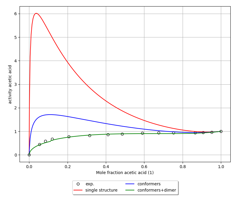
In this example, we’ll investigate the acetic acid/heptane system. In this system, acetic acid prefers to dimerize, making it a good test case to demonstrate the advantages of including multiple forms in a COSMO-RS calculation. We’ll also perform this calculation using only conformers of single acetic acid molecules. Both of these calculations will be compared to the standard COSMO-RS approach using a single structure.

First, we need to generate the .coskf files we need for this calculation. We will consider 3 geometries for acetic acid: 2 unassociated conformers and 1 dimer. These structures are shown below:

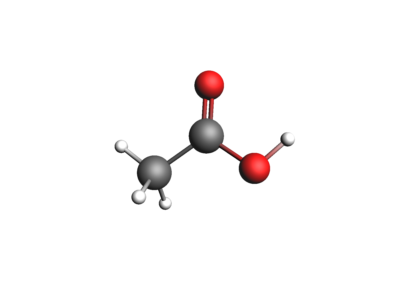
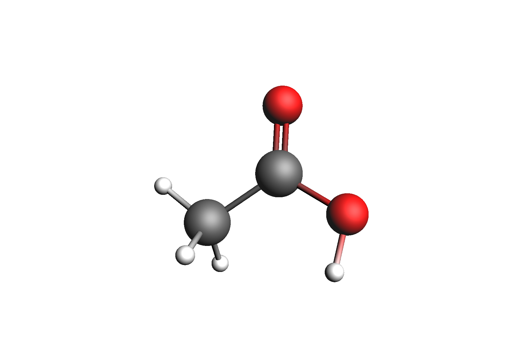
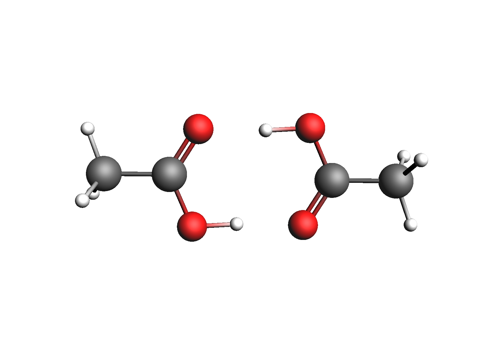
Structures used to represent acetic acid: lowest energy conformer, higher energy conformer, and dimer (clockwise from top left)

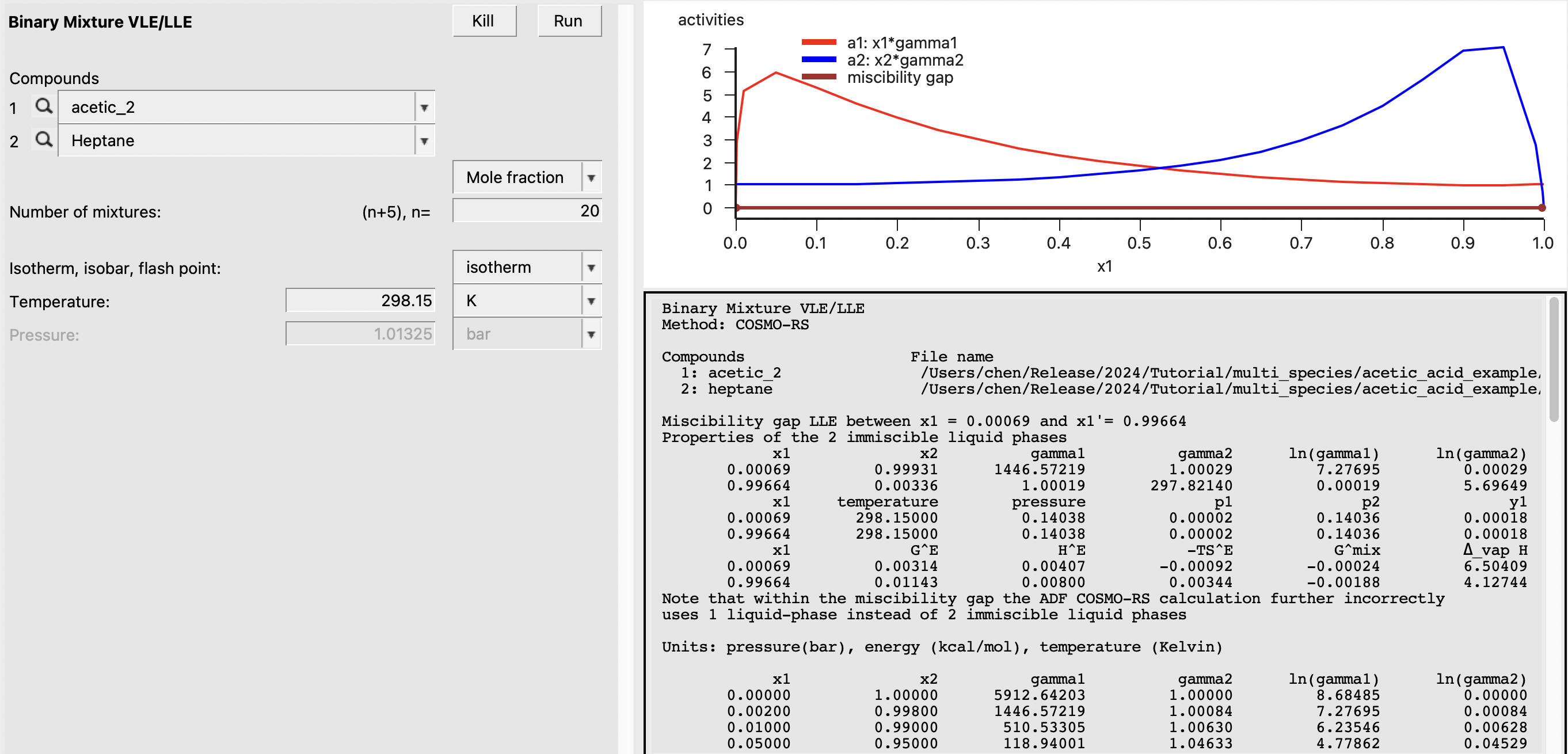
First, we will perform a standard COSMO-RS calculation for reference. In this case, we will intentionally choose the higher-energy conformer to illustrate that the results can be significantly influenced by a poor choice of conformer. An additional advantage of using multispecies compounds is that the lowest-energy conformer is preferred automatically in the calculations and the user does not have to exercise so much caution when selecting structures. To do a standard calculation, we perform the following steps:

Properties → Binary Mixture VLE/LLE

Select acetic_2.coskf or compound 1

Select Heptane for compound 2

Set n to 20

Click Run

Graph → Y Axis → activities

The result of this calculation is the following:

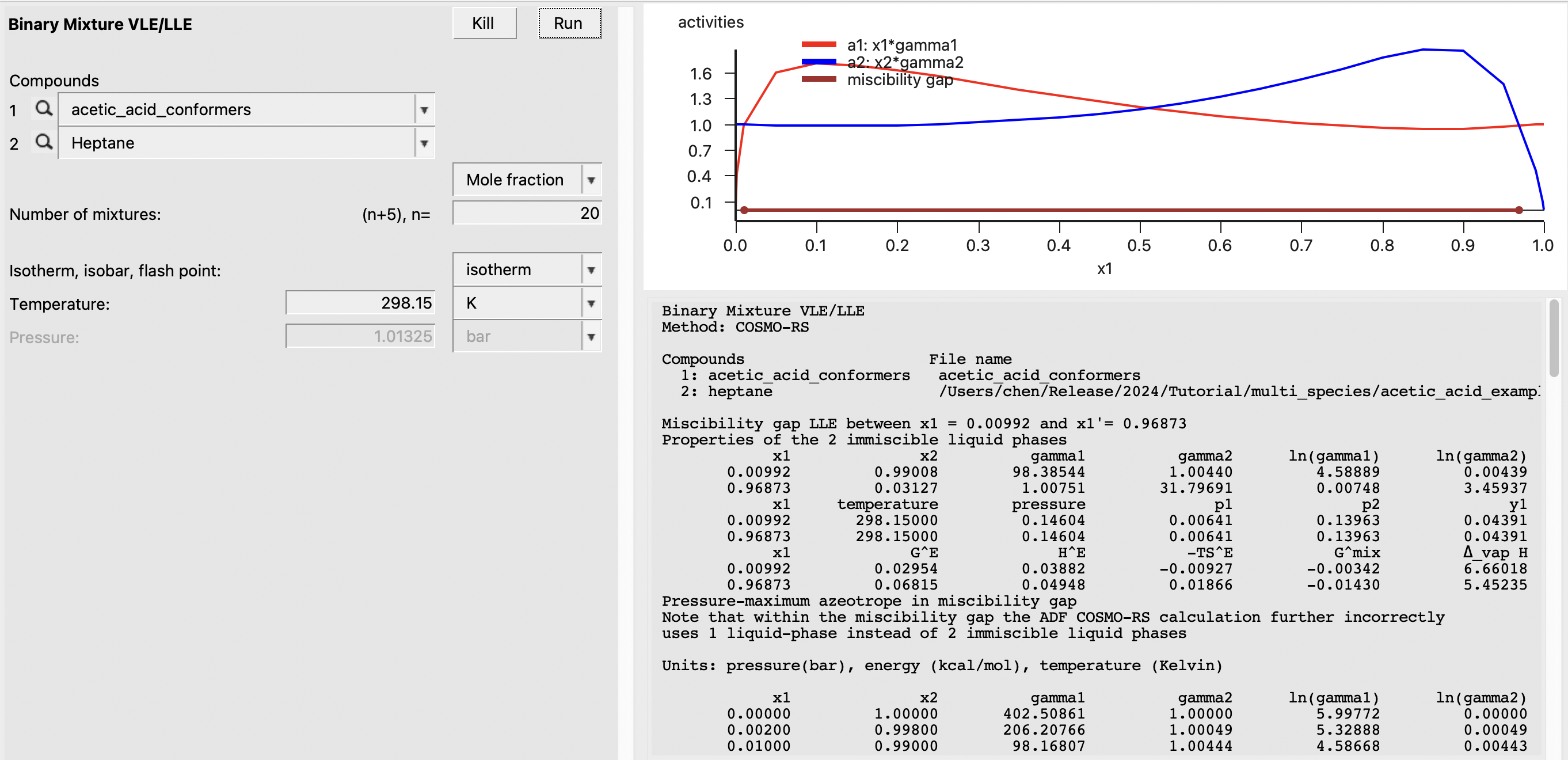
Next, we will perform the calculation considering 2 conformers for acetic acid. This can be done by creating a .multipleform file according to the following:

Compounds → Compound with multiple forms

Add the acetic_1.coskf under conformers

Add the acetic_2.coskf under conformers

Hit save in the top of the multiple forms box

Save as acetic_acid_conformers.multipleform

Now, we perform the same steps as above in the Binary Mixtre VLE/LLE module, except this time we will use the acetic_acid_conformers.multiform instead of acetic_2.coskf.

This should result in the following image:

Finally, we build the .multipleform file acetic acid with the dimer included. These steps are summarized below:

Compounds → Compound with multiple forms

Add the acetic acid conformers under conformers

Add the acetic acid dimer under dimer

Set the Hcorr of the dimer to 9.25

Hit save in the top of the multiple forms box

Save as acetic_acid.multipleform

The GUI should look like the following:

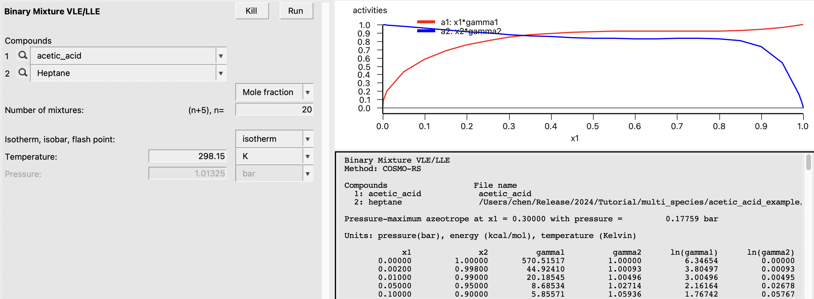
Now, we’ll repeat the same steps as above, this time using the acetic_acid.multipleform file (including the dimer) in place of the previously used acetic acid file.

The result of this calculation is the following:

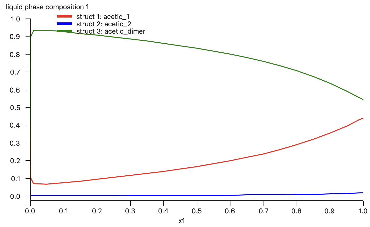
Additionally, we can view the relative amounts of the different forms of acetic acid as a function of mole fraction. To view this, do the following:

Graph → Y Axis → Liquid phase composition 1

This should produce the following:

Finally, we can compare the calculated activities to experimental values 1 among 3 scenarios: (1) using a single structure for acetic acid that is also not the lowest energy conformer; (2) using two conformers for acetic acid; and (3) using both conformers and the dimer.

Solvent association in the diethyl ether/chloroform system

Relevant files for example

.coskf files

In this example, we’ll investigate the effect of an association that takes place in the diethyl ether/chloroform system. This effect is observed because the hydrogen atom in chloroform is electron deficient and forms a H-bond with the oxygen in diethyl ether. We begin this example by generating .coskf files for the three relevant structures: diethyl ether, chloroform, and the associated complex. These files can be created by the user by following the steps outlined in the COSMO result files tutorial . Alternatively, the required coskf files can simply be downloaded using the link above (recommended). The structures used in this example are shown below.

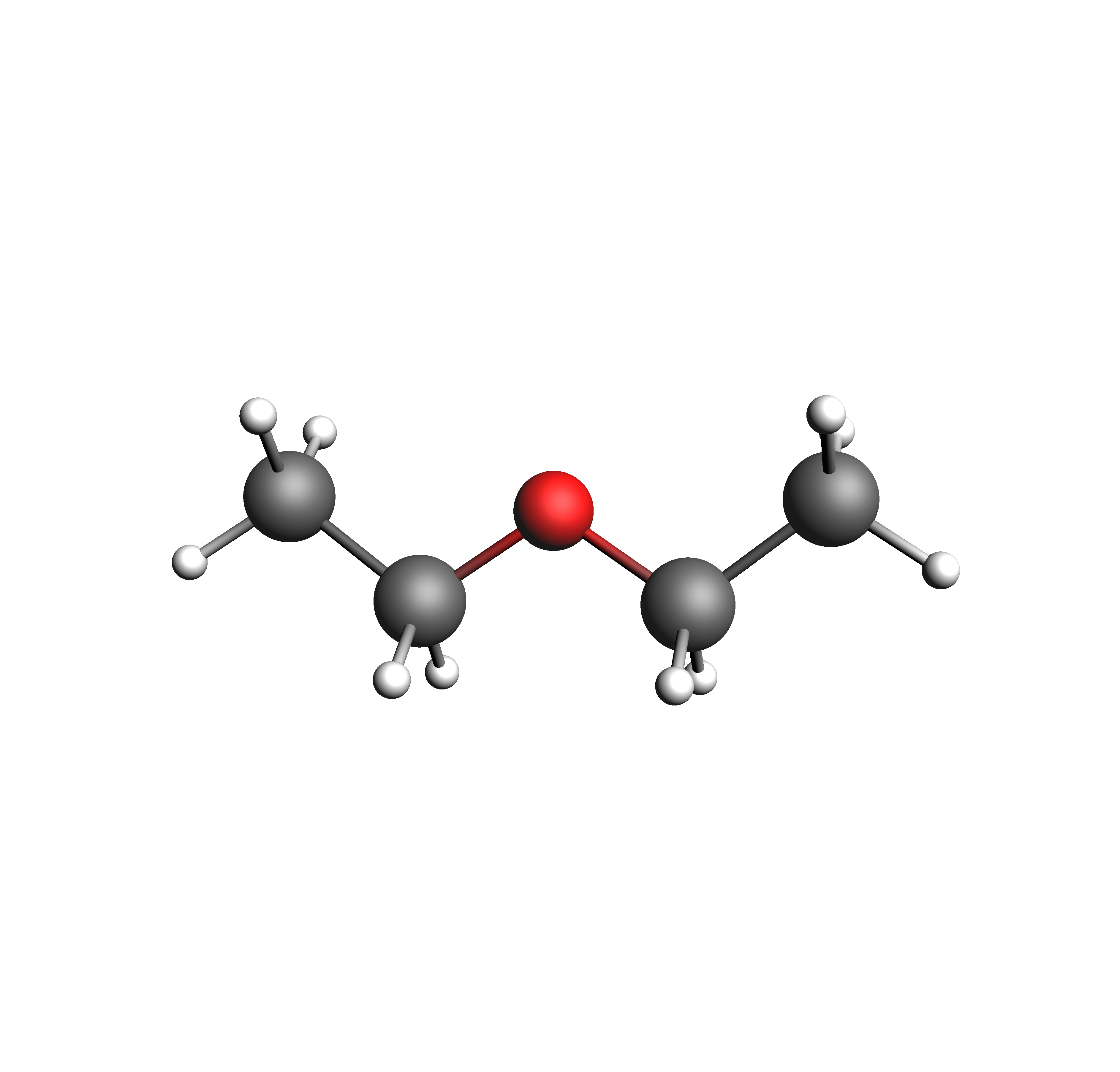
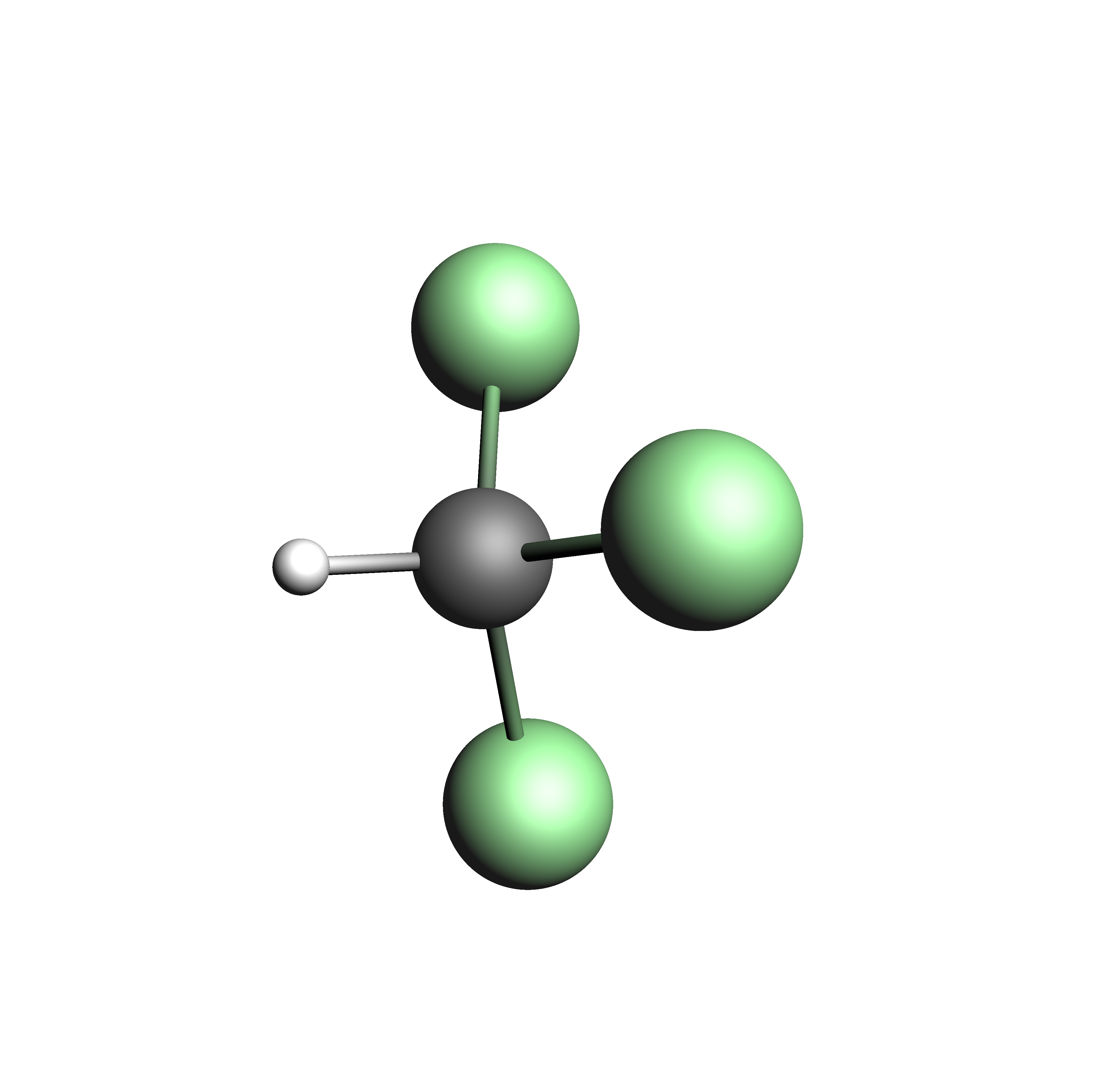
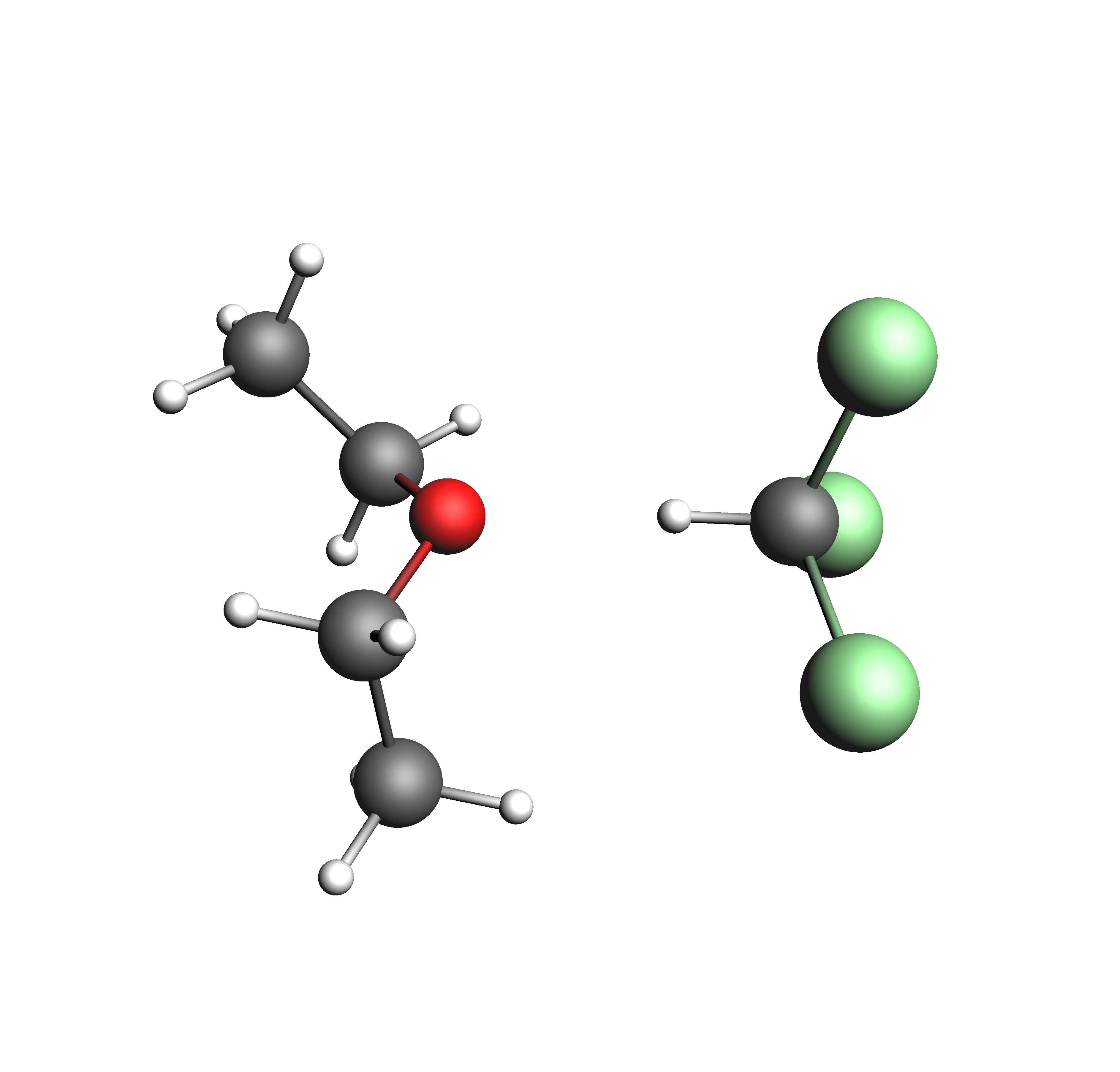
Structures used in the diethyl ether chloroform system: diethyl ether, chloroform, and the associated complex (clockwise from top left)

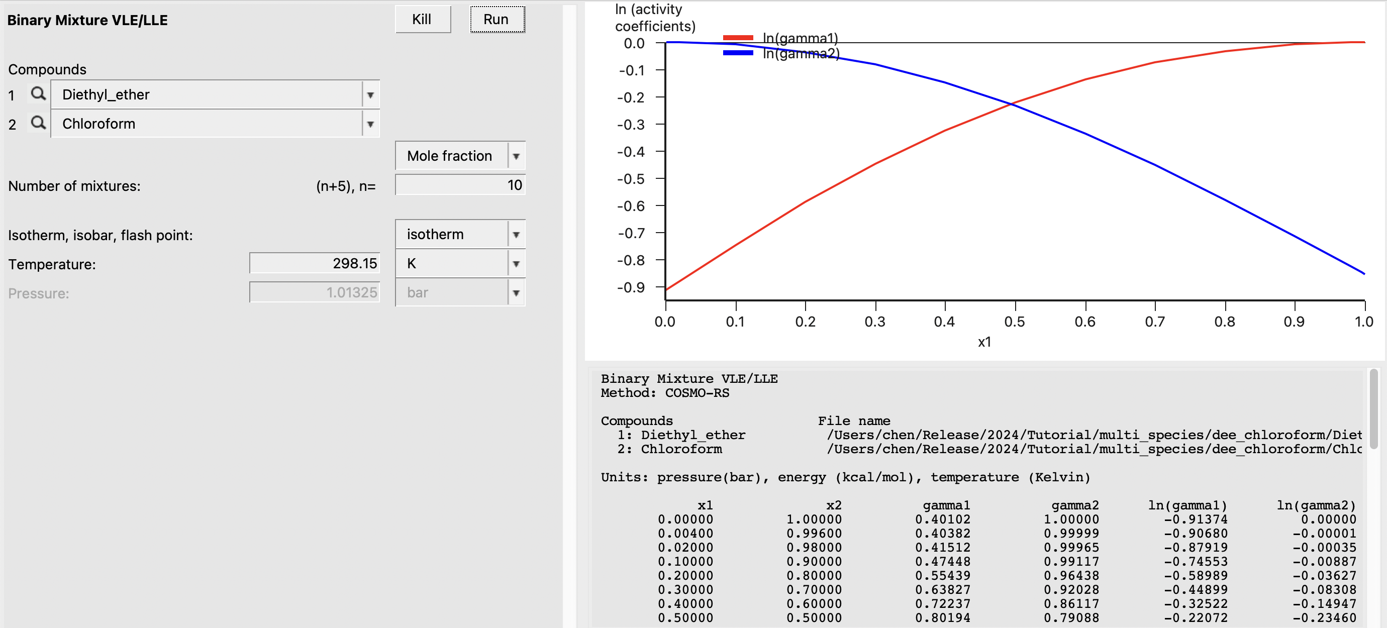
First, we’ll simply consider the system without association. This can be done by performing the following steps:

Input Chloroform.coskf and Diethyl_ether.coskf to the AMS COSMO-RS GUI

Properties → Binary Mixture VLE/LLE

Select Diethyl_ether for compound 1

Select Chloroform for compound 2

Click Run

Graph → Y Axis → ln (activity coefficients)

This should result in the following:

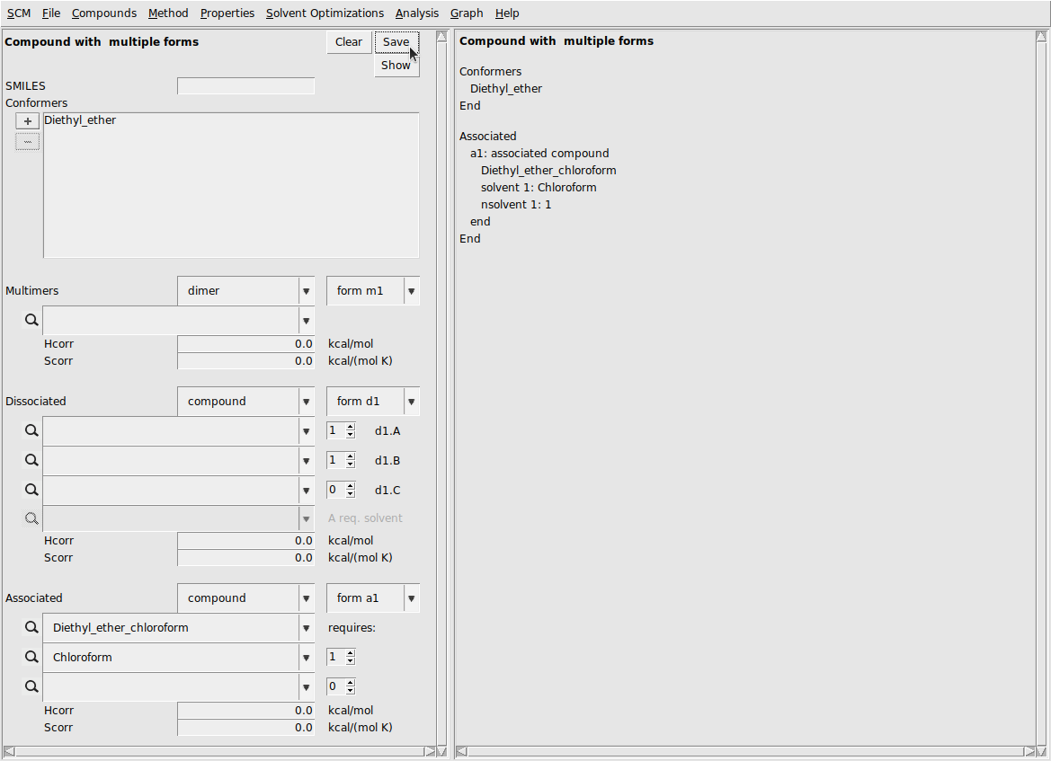
Now, we’ll create a .multipleform file by adding the associated form to diethyl ether (it can also be added to chloroform). This procedure is as follows:

Compounds → Compound with multiple forms

You may need to press ‘Clear’ at the top of the left window

In the conformers section, add Diethyl_ether

In the associated section, add the associated Diethyl_ether_chloroform

Add chloroform to the requires box and make sure the requires value is 1

Save the multipleform file

This should produce the following result:

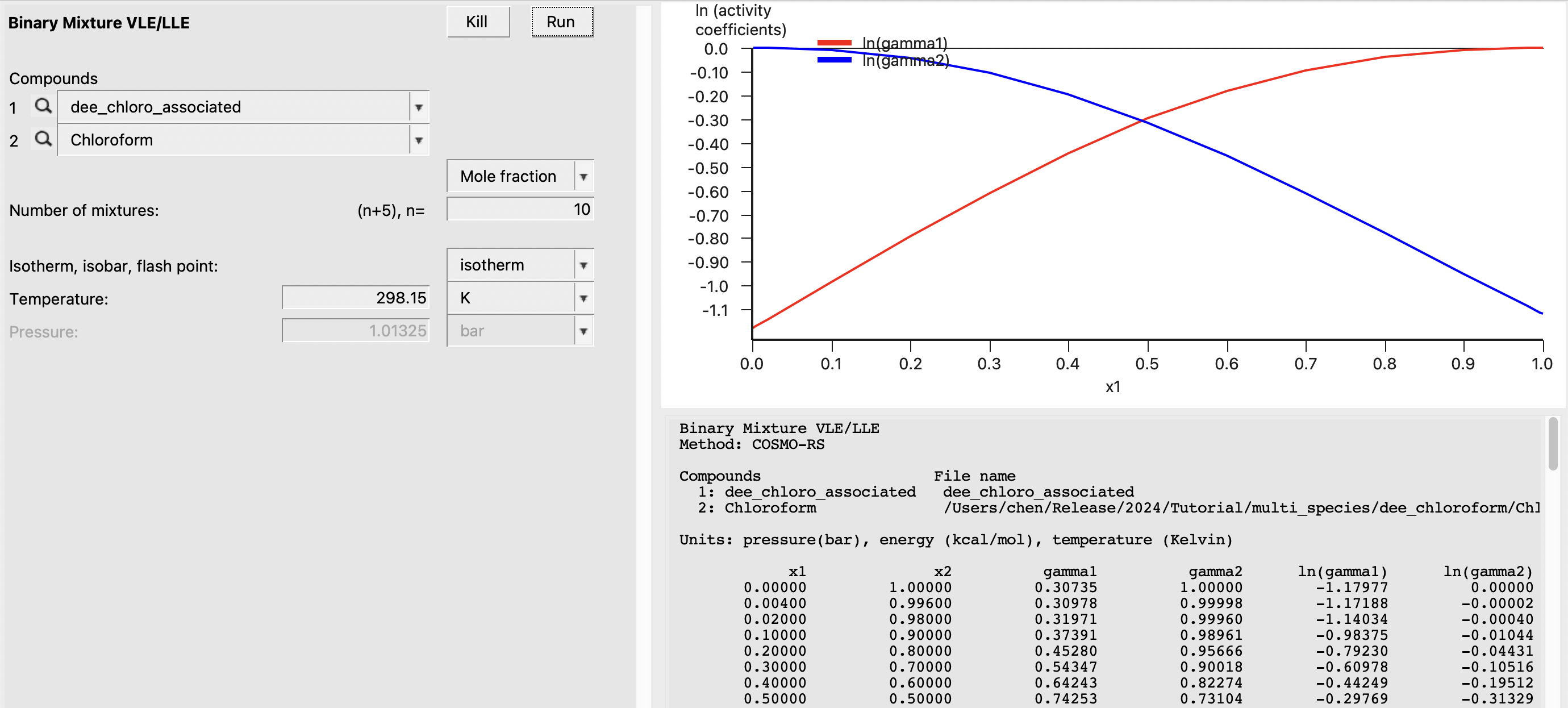
Now, we’ll use the multipleform file in place of the diethyl ether file and repeat the binary mixture calculation.

Input the multiform diethyl ether/chloroform associated complex to the AMS COSMO-RS GUI

Properties → Binary Mixture VLE/LLE

Select the multiform file for compound 1

Select Chloroform for compound 2

Click Run

Graph → Y Axis → ln (activity coefficients)

This should result in the following:

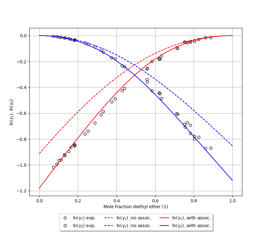
Finally, we can compare the two approaches to experiment 2. We observe that the inclusion of the explicit association greatly improves the agreement with experimental values.

Conformer populations across the chloroform-water phase partition

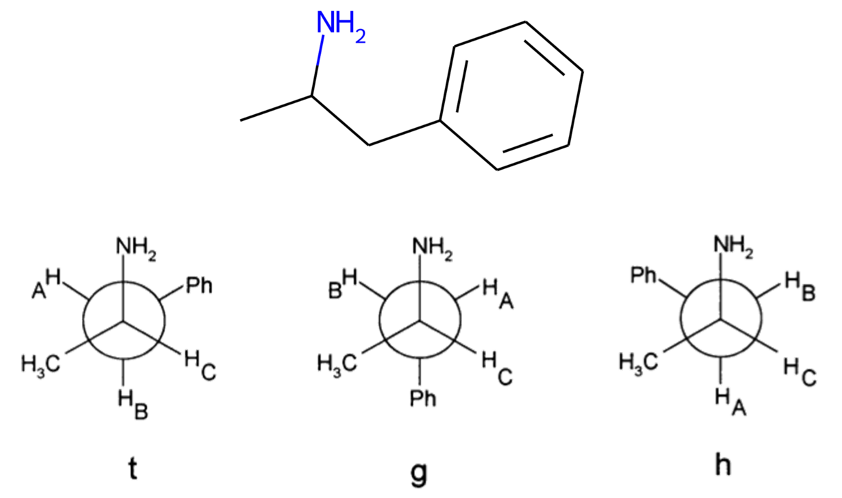
In this example, we will investigate the differences in conformer populations of amphetamine between water and chloroform solvents. Additionally, we will look at how the partition coefficient is affected by accounting for the conformers of amphetamine. Amphetamine has three conformers, denoted in the literature 3 as the t-form, g-form and h-form. These are shown below.

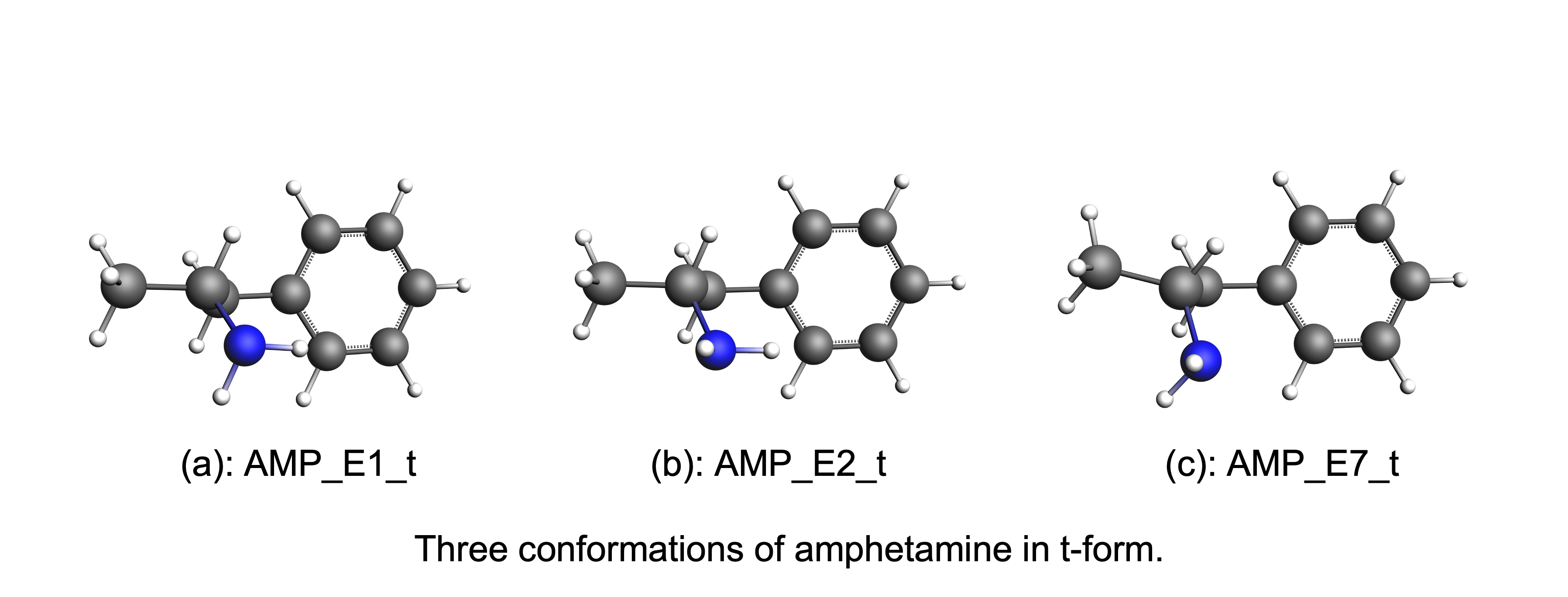
For each conformer we can additionally rotate the C-N bond, producing 3 additional conformers for each of the conformers above. The figure below shows the three conformations of amphetamine in the t-form.

Relevant files for example

.coskf files

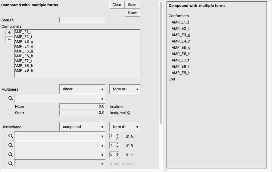
The conformations in this example may be prepared by the user, but for convenience we have included all relevant .coskf files in the link to the right. The filenames refer to the energy in the COSMO phase as well as which conformer is represented. For example, AMP_E1_t is the t-form conformer and has the lowest energy (among the 3 C-N rotamers) while AMP_E9_h is the h-form conformer and has the highest energy. Next, let’s prepare a .multiform file to use with COSMO-RS.

Compounds → Compound with multiple forms

You may need to press ‘Clear’ at the top of the left window

In the conformers section, add AMP_E1_t, AMP_E2_t, … and AMP_E9_h.

Save the multiform file

The GUI should look like the following:

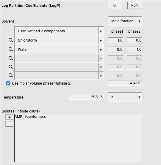
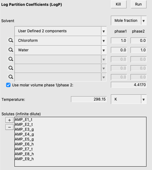
Now, we can set up a logP calculation with the .multiform we just made. This procedure is as follows:

Properties → Partition Coefficient(LogP)

Select User Defined 2 components

Select Chloroform for compound 1

Select Water for compound 2

Add the .multiform file as solute

Set molar volume ratio 4.4170

Click Run

This should result in the following:

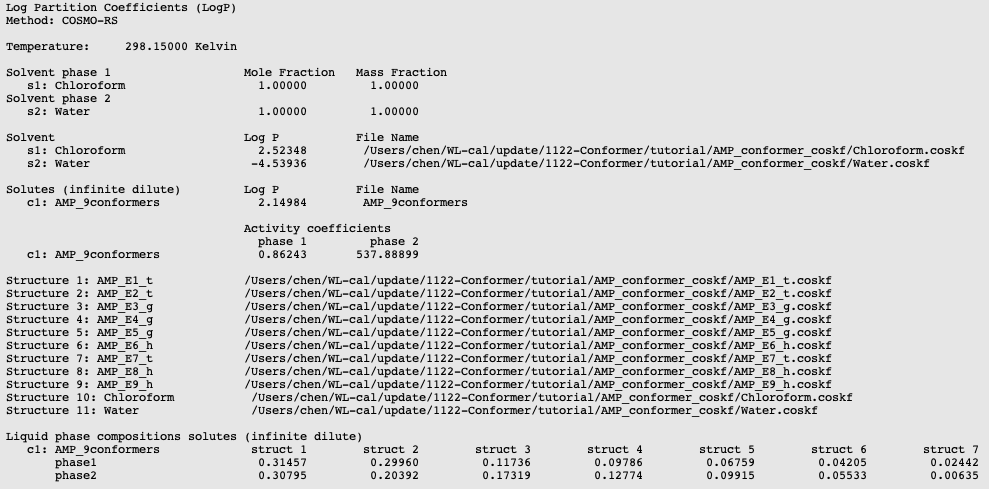
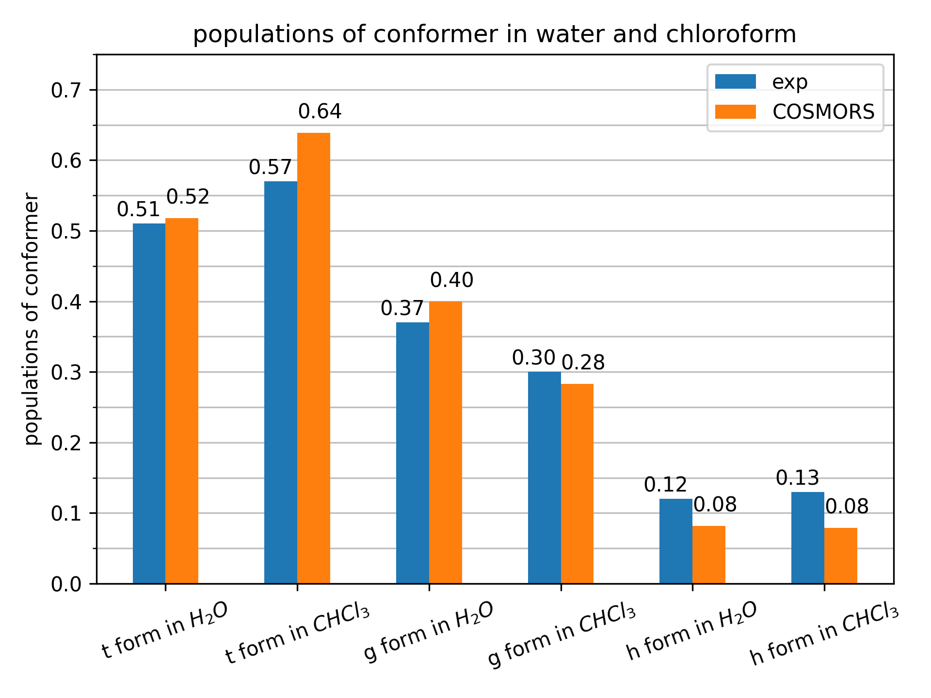
Now, we can sum up the populations of all of the 3 conformations for each of the t-form, g-form, and h-form. Comparing these results to conformer populations derived from H-NMR data 3, we observe good agreement with our predictions. This is shown in the the figure below.

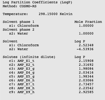
We can additionally do a logP calculation for every individual conformation. Simply delete the .multiform file from the solutes window, add all the individual .coskf files, and then click run. The results show that the calculated logP ranges from 1.98 to 2.92 for the different conformations.

References

1

Lark, Bhajan S., et al. Excess Gibbs energy for binary mixtures containing carboxylic acids. 1. Excess Gibbs energy for acetic acid+ cyclohexane,+ benzene, and+ n-heptane. Journal of Chemical and Engineering Data 29.3 (1984): 277-280.

2

Becker F.; Kiefer M.; Rhensius P.; Schaefer H.D.: Interpretation von Dampfdruckdiagrammen binärer flüssiger Mischungen mit Hilfe von Gleichgewichtsmodellen. Z.Phys.Chem.(München) 92 (1974) 169-192

3(1,2)

Noszál, B., & Kraszni, M. (2002). Conformer-specific partition coefficient: Theory and determination. The Journal of Physical Chemistry B, 106(5), 1066-1068.