COSMO result files
If you already have COSMO result files for all the compounds that you are interested in you can skip this tutorial, without problems of continuity. For example, ADF has a database of COSMO result files, the COSMO-RS compound database ADFCRS-2018.
The purpose of this tutorial is to teach you how to make data for a compound using the ADF program such that it can be read by COSMO-RS. COSMO-RS expects so called COSMO result files, which are results of quantum mechanical calculation using COSMO. In ADF such a COSMO result file is called a TAPE21 (.t21) file, RKF (.rkf), or a COSKF (.coskf) file. For example the COSMO-RS compound database ADFCRS-2018 consists of .coskf files. In other programs such a file could be called a .cosmo file. For example, at https://design.che.vt.edu one may find a database of .cosmo files, which were made with a different program. Note that the optimal COSMO-RS parameters may depend on the program chosen.
Please read through the first GUI tutorial before starting with this tutorial. Even better: try using the AMS-GUI yourself, especially the Getting started Tutorial.
In this tutorial an ADF COSMO result file and a MOPAC COSMO result file will be made. We will also use the program FastSigma to quickly estimate the sigma profile of molecules from SMILES strings.
For ADF COSMO-RS calculations the recommended choice is to use ADF COSMO result files.
For very fast calculations, in which one avoids doing a quantum mechanical calculation for a compound, the FastSigma method is recommended.
Step 1: Start AMSinput
For this tutorial we prefer to work in a separate directory, for example a directory called Tutorial, as was explained in the Getting started Tutorial.
Start AMSjobs (in your home directory), and move to the Tutorial directory:
Next start AMSinput using the SCM menu.
Step 2: Create the molecule
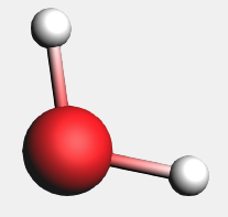
First we construct a water molecule, and preoptimize its geometry:


By symmetrizing the system ADF will use symmetry. Your water molecule should look something like this:
Step 3: ADF COSMO result file
The next step is to optimize the gas geometry using ADF, and perform the ADF COSMO calculation at the optimized gas phase geometry, using Task: COSMO-RS Compound.
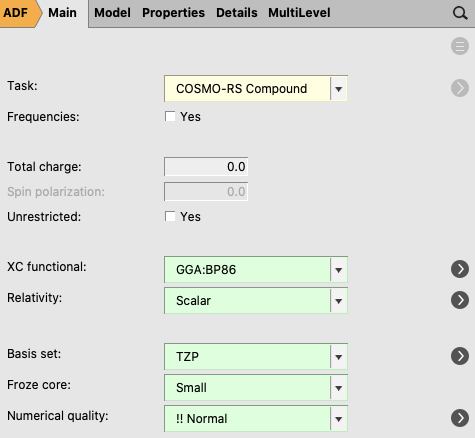
For your information, the proper settings for the gas phase geometry optimization are: the Becke Perdew exchange correlation functional (GGA:BP86), use of the scalar relativistic ZORA Hamiltonian, a TZP small core basis set (for Iodine a TZ2P small core basis set), and an integration accuracy with a normal quality. Like for Iodine, for heavier elements than Krypton, a TZ2P small core basis set is recommended. Note that these settings were used for the optimization of the COSMO-RS parameters.
In the version after AMS2025, an additional densf calculation can be enabled to determine the hydrogen bond center used in COSMO-SAC DHB-ADF MESP method.
 button next to the Task
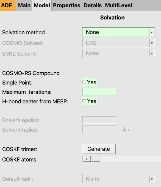
If H-bond center from MESP is set to ‘Yes’, the hydrogen bond center will additionally be determined from the local minima of the molecular electrostatic potential (MESP), calculated from the potentials in the densf calculation.
If Single Point is set to ‘Yes’, a single point calculation will be performed instead of geometry optimization for the gas phase calculation, which is useful when an optimized structure is already available.
With the proper options selected, now run ADF:
Now ADF will start automatically, and you can follow the calculation: AMSjobs will show the progress of the calculation with the last few lines of the logfile.
 button, which will have appeared in the right hand panel, to update the coordinates
Now the geometry of the water molecule is the optimized one, and the ADF COSMO calculation has been performed. The result file water.coskf, which is an ADF COSMO result file, can be used as input for a COSMO-RS calculation.
Note that a .coskf file is not a complete .rkf file. For example, if one has such a .coskf file, only the COSMO surface charge density can be viewed with AMSview. Thus a .coskf file is mostly useful for COSMO-RS calculations.
More details on parameters used in the COSMO calculation can be found in the run script: Details → Run Script. See also the COSMO-RS manual.
Step 4: Lowest Conformer
In standard COSMO-RS theory, one uses one COSMO result file for one molecule in conjunction with the conformer with the lowest energy. Note, however, that sometimes molecules behave in solution in ways that are not accurately captured by the “one-molecule-one-structure” paradigm of standard COSMO-RS theory. For more information, see the tutorial COSMO-RS with multi-species components, where multiple conformers, multimers, dissociated and associated molecules are discussed.
The AMS-GUI does have some basic support for handling conformers. This includes the generation of conformers and the refinement of conformers using different theoretical methods, see the AMS-GUI tutorial on Conformers for more details. In the step in this tutorial where the structures of the conformers are refined, one can use ADF with the Task ‘COSMO-RS Compound’. Next one can select the conformer with the lowest energy to be used as an ADF COSMO result file.
Note that this step does not involve a calculation, but only shows one way to find the lowest conformer.
Alternatively, you can generate the lowest conformer and multiple conformers by utilizing the ADFCOSMORSCompound class and ADFCOSMORSConfJob class through Python scripting. You can find more information and examples in the documentation links provided: ADFCOSMORSCompound class and ADFCOSMORSConfJob. Before running the Python script, please ensure that you have completed the necessary environment setup by referring to the Getting Started with scripting.
Step 5: Polymers with ADF
The AMS-GUI supports the making of a polymer. However, the calculation of a full polymer is very expensive. Instead of this very expensive calculation, here an “average monomer” COSMO result file is calculated. The full polymer result could then be calculated by multiplying the “average monomer” result by a factor equal to the number of repeat units in the polymer.
In this step ADF is used to generate a COSMO result file for a polymer.
One can also use the approximate, but much faster, FastSigma method, described in step 7.
Here, a trimer is calculated from 3 units of the monomer, in which the trimer is capped with 2 methyl groups. Next an ADF COSMO result file is generated, in which only the COSMO charges of the center monomer will be used in the COSMO-RS calculations.
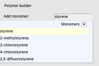
This will create a Polystyrene monomer. The 2 dummy atoms will later be replaced with 2 other monomers to form a Polystyrene trimer.
Next we will not use the Polymer builder window, but instead use a specialized button that generates a trimer, adds 2 methyls as capping groups, and selects the center monomer atoms as so called ‘COSKF atoms’.
If one would select File → Run an “average monomer” COSMO result file would be created, which an be used for polymer calculations. The calculation can take up quite some time, therefore we skip this part in this step.
Step 6: MOPAC COSMO result file
Note this step is presented here only for completeness. One can skip this step, since we do not recommend to use MOPAC to generate COSMO result files.
MOPAC is a faster method than ADF for the generation of COSMO result files. However, we recommend to use the FastSigma program described in the next step, if you want get an estimate of a COSMO result file very quickly and which has a better quality.
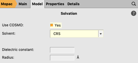
A MOPAC COSMO result file can be created in almost the same way as an ADF COSMO result file. We will change the program from ADF to MOPAC, and select the COSMO solvation method.
 →
→ 
For sake of clarity we will save the COSMO calculation under a different name, and run the calculation
button, which will have appeared in the right hand panel, to update the coordinatesAfter the calculation has finished the file water_mopac.results/mopac.coskf, which is a MOPAC COSMO result file, can be used as input for a COSMO-RS calculation.
Note that MOPAC is a semi-empirical quantum chemistry program, whereas ADF is based on density functional theory (DFT). Thus the MOPAC COSMO result files will not be of the same quality as the ADF COSMO result files.
Step 7: FastSigma: estimating sigma profiles for use with COSMO-RS/-SAC
FastSigma is a program that estimates information in a COSMO result file without doing an expensive DFT calculation. Practically speaking, this that in the timeframe of milliseconds, FastSigma can estimate a sigma profile and other required molecular descriptors used to perform COSMO-RS/-SAC calculations.
See also
The FastSigma Documentation is a useful resource for additional calculation types and more general information.
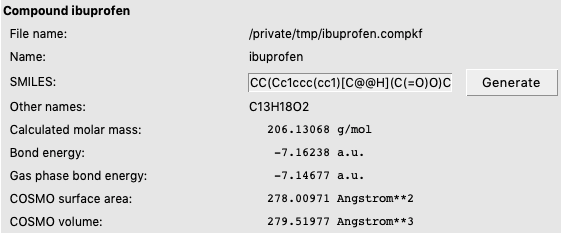
In the GUI, FastSigma can be used for compounds with a SMILES string or an .xyz file. In this example, we use Ibuprofen, which is represented in the SMILES string CC(Cc1ccc(cc1)[C@@H](C(=O)O)C)C.
Note that for a polymer one would need as input a so called CurlySMILES string, which for example, for Polystyrene is C{-}C{n+}(c1ccccc1), see the COSMO-RS polymers tutorial for more details.
CC(Cc1ccc(cc1)[C@@H](C(=O)O)C)C for Ibuprofen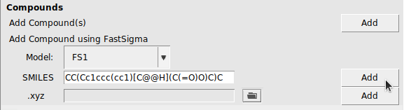
In the right part of the COSMO-RS GUI window one should see something like:
FastSigma does not create a COSMO surface, but creates a so called sigma-profile, which can be used in COSMO-RS calculations. The parameters in FastSigma are fitted to COSMO-RS sigma-profiles of organic closed shell neutral molecules. The created sigma-profile can not be used in COSMO-SAC calculations. The created file contains a SMILES string, thus it can be used in UNIFAC calculations. Note that is is not recommended to be used for radicals or charged molecules.
Important
To use the SG1 method instead of FS1, users will have to first download the Subgraph Sigma Profile Estimation (SG1) Database (molsg_sg1db) using the AMS Package Manager.
One can visualize the molecule in 2D (a .html file will be created) with
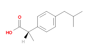
Openbabel is used to translate the SMILES string into a picture.