Overview: properties
How the properties are calculated and definitions used can be found in the section Calculation of properties in the COSMO-RS manual.
Step 1: Start AMScrs
For this tutorial we assume that you know how start AMScrs and how to add compounds. Like in tutorial 2 we ask you to add the compounds water, methanol, ethanol, and benzene. One can do this, for example, by opening the .crs file that was created in tutorial 2. Save the file as tutorial3.crs.
Alternatively on a Unix like system one may copy the COSMO result files (water.coskf, methanol.coskf, ethanol.coskf, and benzene.coskf) in the directory $AMSHOME/examples/COSMO-RS/Parameters_and_Analysis to an empty directory and enter the following command in this directory where the COSMO result files are present:
$AMSBIN/amscrs benzene.coskf ethanol.coskf methanol.coskf water.coskf &
Note that one has to set the number of ring atoms for the benzene compound. This is set to the correct value in the benzene .coskf file in the CRS database, but users will have to set (or estimate) this manually if they generate their own .coskf file.
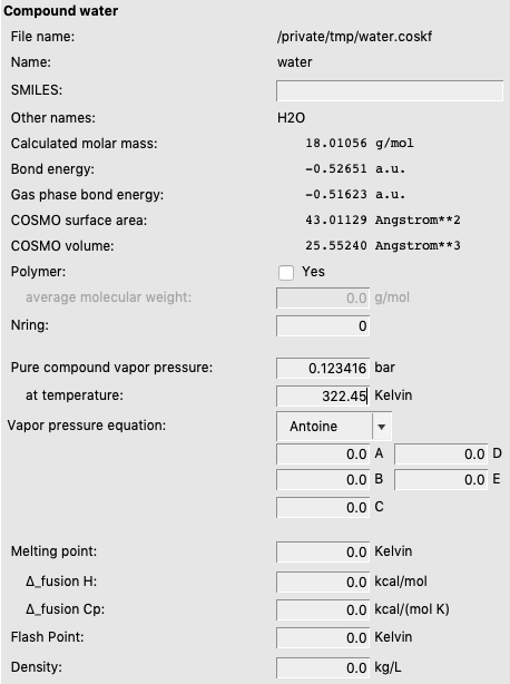
In the compounds window one can also set the vapor pressure of the pure compounds at a given temperature, or set the Antoine parameters. If these values are not specified (if they are zero) then the pure compound vapor pressure will be approximated using the COSMO-RS method. This is relevant, for example, for the calculation of the (partial) vapor pressures of mixtures, calculation of boiling points of mixtures, and calculation of Henry’s law constants.
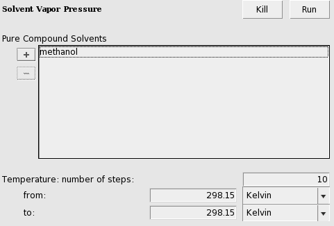
Step 2: Vapor pressure
The vapor pressure of a solvent at different temperatures can be calculated with Properties → Vapor Pressure Pure Solvents or Properties → Vapor Pressure Mixture.
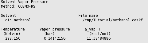
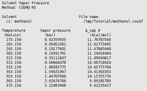
In this case the result is a table with one entry:
In this case the result is a graph and a table. The graph can be edited to change the general appearance and units. Graph editing options can be accessed by clicking outside of the plot, so in the area around the left or bottom axes. Changing a few settings, the graph may look like the following:
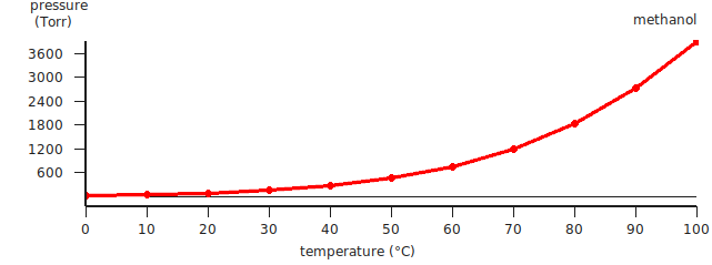
In this case COSMO-RS predicts a vapor pressure of about 0.61 bar (around 455 Torr) at 323.15 K (50.0 °C) for the pure liquid methanol.
Step 3: Boiling point
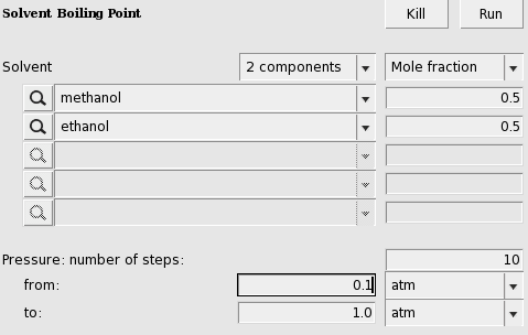
The boiling point of a solvent at different pressures can be calculated with Properties → Boiling Point Pure Solvents or Properties → Boiling Point Mixture.
In this case the result (may take several seconds) is a graph and a table.
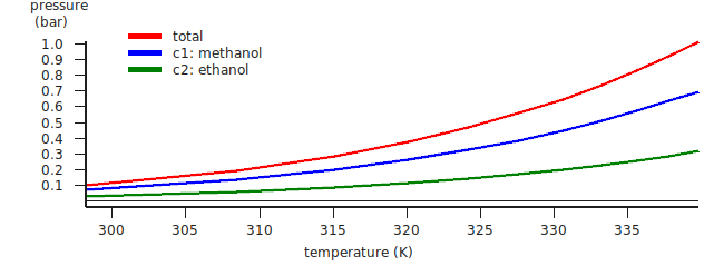
The red curve is the total vapor pressure, the blue curve the partial methanol vapor pressure, and the green curve is the partial ethanol vapor pressure. The table gives the numerical values.
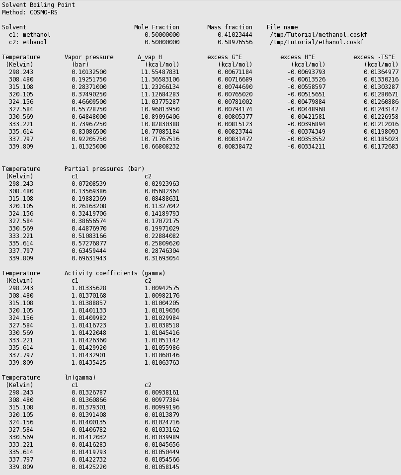
Thus in this case COSMO-RS predicts a boiling point of 339.8 K (66.7 °C) at 1 atm. for this mixture of 50% mole fraction methanol and 50% mole fraction ethanol. At this temperature COSMO-RS predicts that the vapor consists about 69% of methanol.
Using Graph → Y Axes → one can view different properties in the graph, like activity coefficients and excess energies.
Step 4: Flash point
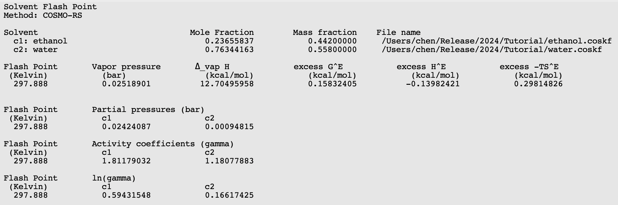
The flash point of a mixture can be calculated with Properties → Flash Point, if pure compound flash points are given as input.
Here we mix equal volumes of water (assuming a density of 0.997 kg/L) and ethanol (assuming a density 0.789 kg/L). For a flash point calculation, the pure compound flash points are needed as input, since COSMO-RS does not predict pure compound flash points. The AMS COSMO-RS module uses Le Chatelier’s mixing rule to calculate the flash point of a mixture.
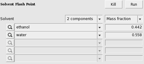
In this case the calculated flash point will be close to 25 °C.
Step 5: Activity coefficients, Henry coefficients, Solvation free energies
The activity coefficients a solvent and the activity coefficients of infinitely diluted solutes in a solvent can be calculated with Properties → Activity coefficients. At the same time Henry coefficients and solvation free energies will be calculated.
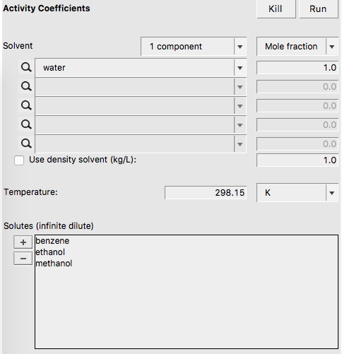
If one does not supply a density of the solvent in the input, the program calculates the density of the solvent by dividing the mass of a molecule with its COSMO volume. Note that the calculated activity coefficients do not depend on this density. One may improve the results for the calculation of the Henry constants, by selecting a compound in the List of Added Compounds, and include pure a compound vapor pressure at a given temperature.
The result of the calculation is given in the form of a table.
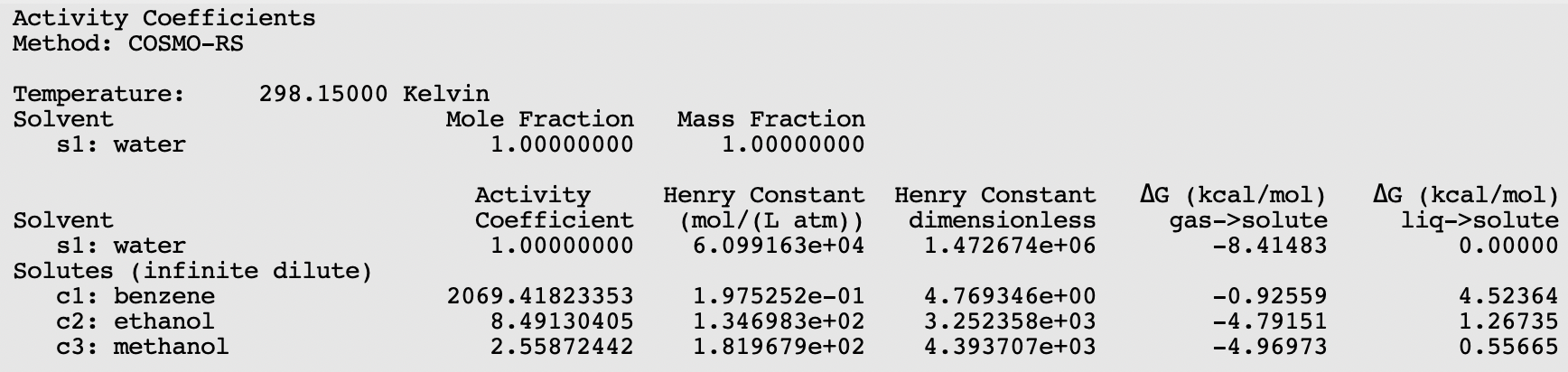
Relevant for the calculation of the Gibbs free energy of solvation ΔG from the gas phase to the solvated phase is the reference state, used here is 1 mol/L in both phases.
Step 6: Partition coefficients (log P)
Preset Octanol/Water, Benzene/Water, Ether/Water, Hexane/Water
The partition coefficients (log P) of infinitely diluted solutes in a mixture of two immiscible solvents can be calculated with Properties → Partition Coefficients (LogP). There are presets for the calculation of Octanol/Water, Benzene/Water, Ether/Water, and Hexane/Water partition coefficients. The presets use compounds that are present in $AMSHOME/atomicdata/AMSCRS.
First the preset Octanol/Water is used.
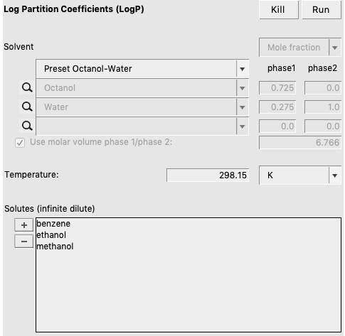
In case of partly miscible liquids, like the Octanol-rich phase of Octanol and Water, both components have nonzero mole fractions. The preset also gives a value for the molar volume quotient of the two solvents.
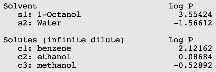
The result of the calculation is given in the form of a table.
User defined
A user can also define 2 phases of a mixture of two (or three) immiscible solvents.
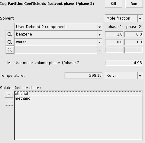
Here an input value is used for the volume quotient of the two solvents. If one does not include such value, the program will use the COSMO volumes to calculate the volume quotient. The COSMO volumes can be found by selecting a compound in the List of Added Compounds.
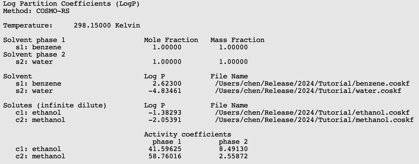
The result of the calculation is given again in the form of a table.
Step 7: Solubility
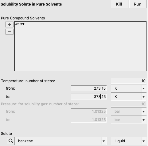
The solubility of a solute in a solvent can be calculated with Properties → Solubility in Pure Solvents or Properties → Solubility in Mixture. The solute can either be a liquid, solid, or gas.
Solubility liquid in a solvent
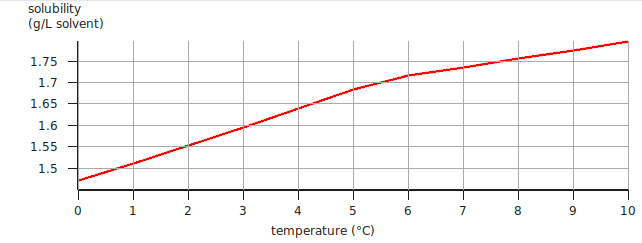
First the solubility of benzene in water for a range of temperatures.
If a range of temperatures is requested a graph is shown.
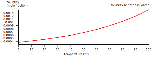
A major assumption made in here in liquid-liquid solubility calculations is that at the point of liquid-liquid equilibrium, the solute will co-exist in a pure liquid phase. In many cases, this is an invalid assumption. This can lead to particularly high errors if the solubility of the solvent in the liquid is high. A better way to perform a liquid-liquid equilibrium calculation and look at the miscibility gap. An example is given for the calculation of the miscibility gap in the binary mixture of Methanol and Hexane.
Note that experimentally benzene is a solid below 5.5 °C, and a gas above 80.1 °C. This has not been taken into account in this case. See the next examples.
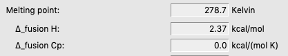
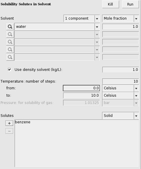
Solubility solid in a solvent
For the solubility of a solid compound in a liquid, it is necessary to include the melting point, the enthalpy of fusion, and the Δ heat capacity of fusion of the pure compound. The Δ heat capacity of fusion is optional (and often hard to find experimental numbers for), as it often makes little difference in these calculations. These required values can be input for each compound from the Compounds → List of Added Compounds menu. Here, some experimental values will be included for benzene (see, for example, https://en.wikipedia.org/wiki/Benzene).
Also an experimental value for the density of water will be used:
After editing the appearance of the graph, the result may look like the following:
Solubility gas in a solvent
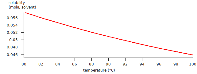
For the solubility of a gas one should the change the ‘Liquid’ popup menu in ‘Gas’ and enter a partial pressure in the ‘Pressure’ field.

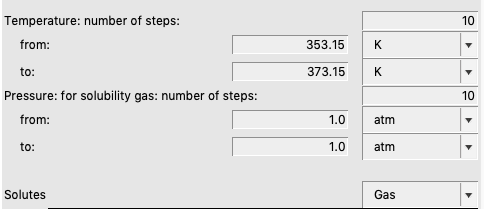
A graph (and table) is shown, which after some manipulations could look like:
The solubility of a gas in a solvent can also be calculated using Henry’s law, which is valid for ideal dilute solutions.
The calculated Henry constant for benzene (infinite dilute) in water will be close to 0.049 mol/(L atm) at 90 °C (363.15 K).
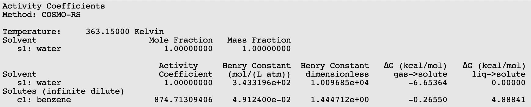
Note that for benzene, in the compounds window, the vapor pressure was entered at 353.3 Kelvin. If these values are not specified (i.e. if they are zero) then the vapor pressure will be approximated using only the COSMO-RS method. This is relevant for all properties where the vapor pressure plays a role, thus it is relevant for the calculation of Henry’s law constants and relevant for the calculation of the solubility of a gas in a solvent.
Step 8: Binary mixtures VLE/LLE
A phase diagram of a mixture of two components can be calculated with Properties → Binary Mixture VLE/LLE. The binary mixture will be calculated for a list of molar fractions between zero and one. This can be done at constant temperature (isothermal) or at constant vapor pressure (isobaric).
Isothermal
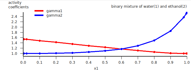
A binary mixture is calculated in which the pure compound vapor pressures are approximated using the COSMO-RS method.
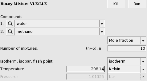
An activity coefficient plot for water(1) and methanol(2) will be shown.
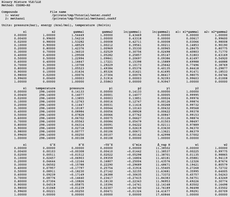
The results of the calculation are also given in the form of a table, which shows the molar (and mass) fraction of each compound in the liquid, the activity coefficients, the activities, the temperature, the total and partial vapor pressures, the molar fraction of each compound in the vapor (y), the excess Gibbs free energy GE , the excess enthalpy HE (calculated with the Gibbs-Helmholtz equation), the excess entropy of mixing -TSE , the Gibbs free energy of mixing Gmix , the enthalpy of vaporization Δvap H (calculated with the Clausius-Clapeyron equation).
These values can also be shown in a graph. The property for the x- and y-axes can be selected from the ‘Graph’ Menu. For example, a graph of the excess energies can be shown by:
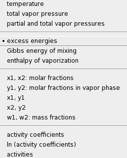
A plot of the excess energies will be shown.
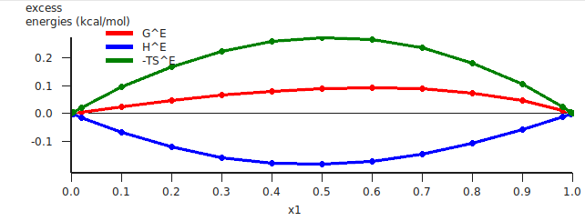
The red curve is the excess Gibbs free energy GE , the blue curve is the excess enthalpy HE , and the green curve is -T times the excess entropy SE .
Isothermal, input pure compound vapor pressure
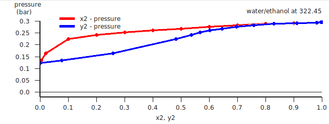
A binary mixture is calculated with input data for the pure compound vapor pressures. These can be, for example, experimentally observed pure compound vapor pressures. Note that the calculated partial and total vapor pressures will now depend on these input pure compound vapor pressures.
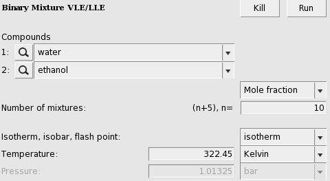
A vapor liquid equilibrium (VLE) diagram for water(1) and ethanol(2) will be shown.
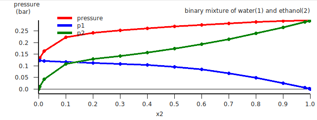
The red curve is the total vapor pressure, the blue curve is the partial water vapor pressure, and the green curve is the partial ethanol vapor pressure. One can also change the x and y axes, for example:
Isothermal, miscibility gap, LLE
Water and benzene do not mix well, thus there will be a miscibility gap.
In this case, a liquid-liquid equilibrium (LLE) is calculated. It is important to note that the built-in method estimates isoactivity between two immiscible liquid phases by interpolating the calculated activities. Therefore, it provides a fast estimate, but the results are less accurate than those from the full LLE solver especially when the number of mixture points is too small.
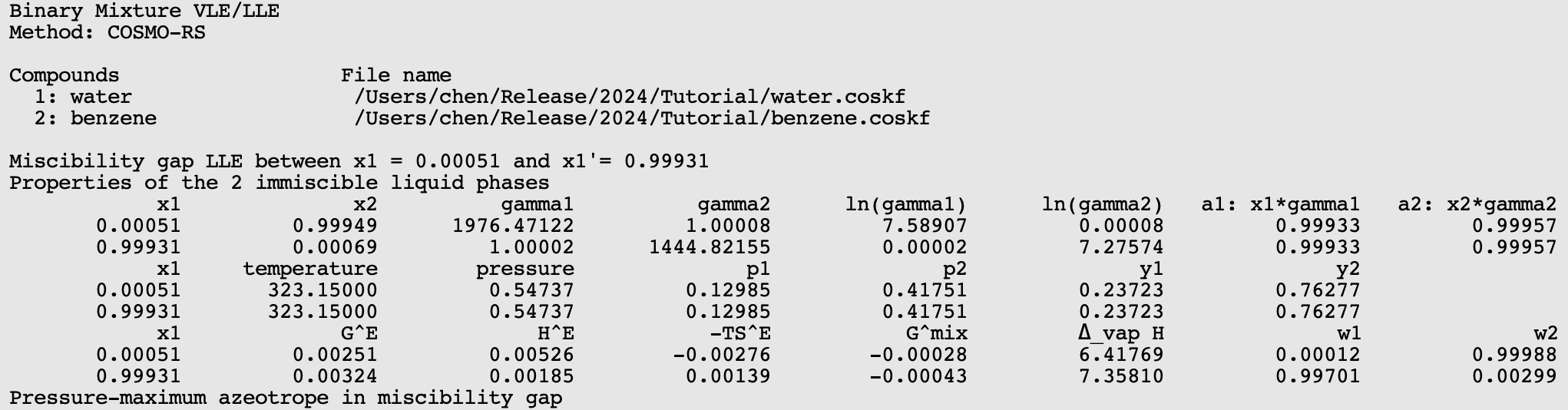
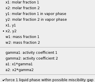
If the check box Graph → X axes → force 1 liquid phase within possible miscibility gap is deselected, then results will be shown in the graph and table only for those compositions of the mixture, which are outside of the miscibility gap. If the check box Graph → X axes → force 1 liquid phase within possible miscibility gap is selected, then results will be shown also within the miscibility gap, with the unphysical conditions that the two liquids are forced to mix.
Isobaric
A binary mixture is calculated in which the pure compound vapor pressures are approximated using the COSMO-RS method if the input values for the pure compound vapor pressures are zero. Alternative one can click a check box in the ‘Method’ Menu.

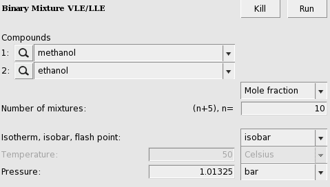
The calculated boiling points (may take several seconds) for a binary mixture of methanol(1) and ethanol(2) will be shown.
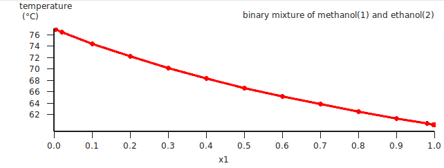
If one clicks in the graph window at the left or below the axes, a popup window will appear in which one can set details for the graph window. In the graph above the ‘Units’ for the ‘Left Y Axes’ were chosen to be ‘Celsius’.
Next the same binary mixture is calculated in which experimental pure compound vapor pressures are used.

The calculated graph will not look very different, but it will be more accurate.
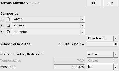
Step 9: Ternary mixtures VLE/LLE
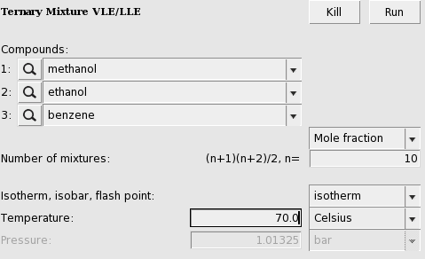
A phase diagram of a mixture of three components can be calculated with Properties → Ternary Mixture VLE/LLE. The ternary mixture plot will be calculated by iterating over possible values of molar (or mass) fractions for each of the compounds. This can be done at constant temperature (isothermal) or at constant vapor pressure (isobaric).
In this step we will use experimental boiling points as input.
Isothermal
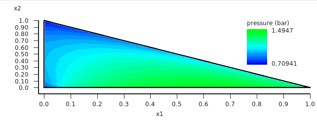
The result will be a graph and a table. In the table one can find the results of the calculation at 55 (=(n+1)(n+2)/2, with n=10) different compositions. At those compositions the table shows the molar (and mass) fraction of each compound in the liquid, the activity coefficients, the activities, the temperature, the total and partial vapor pressures, the molar fraction of each compound in the vapor (Y), the excess Gibbs free energy GE , the excess enthalpy HE (calculated with the Gibbs-Helmholtz equation), the excess entropy of mixing -TSE , the Gibbs free energy of mixing Gmix , the enthalpy of vaporization Δvap H (calculated with the Clausius-Clapeyron equation).
These quantities can also be shown in the graph as a colormap, in which the color represents the value of the quantity at a certain composition. On the X axes of the graph one can choose the molar (or mass fraction) of one of the compounds, on the Y axes one can choose the molar (or mass fraction) of another compound. The molar (or mass) fraction of the third compound is then fixed, since the sum of the fractions is 1.
In this case the colormap shows the total vapor pressure:
One can improve the quality of the graph by increasing the number of compositions. Note that the number of different compositions for n=20 is 231 (=(n+1)(n+2)/2).
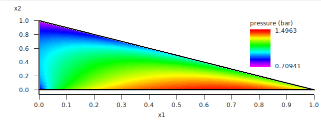
If one clicks in the graph window at the left or below the axes, a popup window ‘Graph details’ will appear in which one can set details for the graph window. If one chooses in the ‘Z Colormap’ part of this popup window as the minimum color magenta, as maximum color red, use 100 as number of colors, and change the minimum and maximum values, then the graph could look like this:
Isobaric
Note that isobaric calculations are more expensive than isothermal calculations. Thus the following example takes quite some time, since again for n=20 the number of different compositions is 231.
The result will be a graph and a table. Note that this may take some time, since isobaric calculations are more expensive than isothermal calculations. Click in the graph window at the left or below the axes. If one chooses in the ‘Z Colormap’ part of the ‘Graph details’ as the minimum color blue, as maximum color red, use 5 as number of colors, change the unit to Celsius, and change the minimum and maximum values to 60 and 80 Celsius, then the graph could look like this:
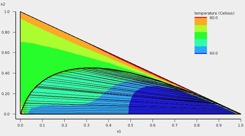
In addition to the colormap of the temperature, an approximate miscibility gap of the ternary mixture is shown in the graph. In this case, within the miscibility gap there are two immiscible phases of the liquid in equilibrium. The composition of the two phases, which are in equilibrium, can be found at the end points of the tie line that are drawn. The calculated temperatures within the miscibility gap are calculated with the unphysical condition that the three liquids are forced to mix, thus these calculated temperatures (and other quantities) within the miscibility gap should not be used. By inspection of the graph, one can observe that the calculated minimum boiling point (azeotrope) is around 68 °C.
Step 10: A composition line between solvents s1 and s2
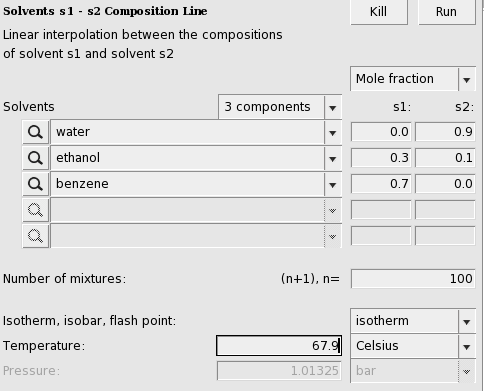
A phase diagram of a mixture of two solvents, which both could be mixtures, can be calculated with Properties → Solvents s1 - s2 Composition Line. The mixture will be calculated for a list of molar (or mass) fractions of the solvents between zero and one, and the compositions of solvent 1 and solvent 2 are linearly interpolated. This can be done at constant temperature (isothermal) or at constant vapor pressure (isobaric).
In this step we will try to investigate one of the tie lines of the ternary mixture of water, ethanol, and benzene in more detail. An attempt is made to use the tie line on which ends the calculated minimum boiling point is found, see the tie line which is below the black line in the next picture:
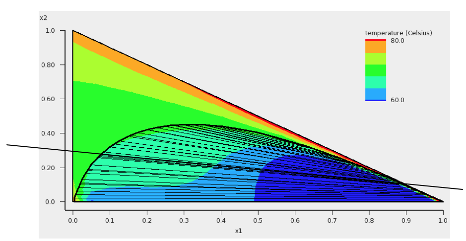
The compositions of solvents s1 and s2 are chosen where the black line in the picture above crosses the boundary of possible compositions. This means that solvent s1 and solvent s2 are mixtures of 2 compounds. Again experimental boiling points are used in the calculation.
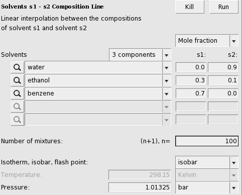
The result will be a table and a graph.
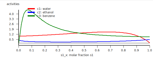
The activities of the pure compounds should be equal at the end point of a tie line a1 = a1′,a2 = a2′, and a3 = a3′. If we look at the graph with close inspection this is approximately true for the molar fraction of solvent s1 with (approximately) s1_x = 0.007 and s1_x′ = 0.91. At a molar fraction of 0.91 of solvent s1 the calculated temperature is approximately 67.9 °C (341.05 K).
Next we will use this temperature of 67.9 °C and look at the Gibbs free energy of mixing. This will also give information about the miscibility gap.
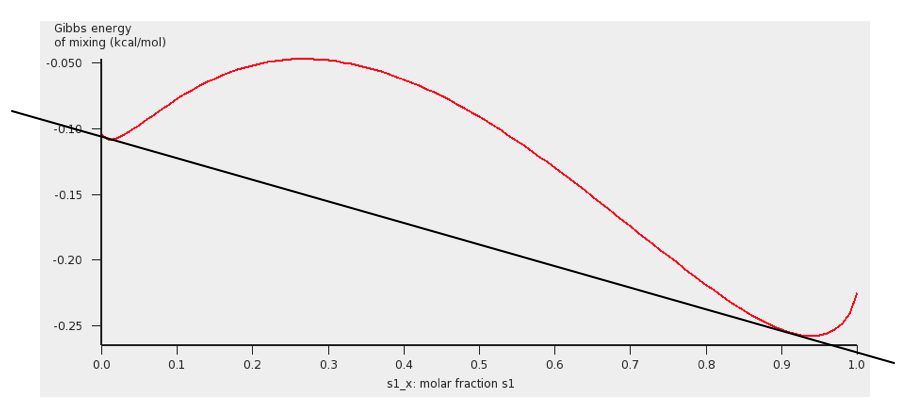
The black line was added to show the miscibility gap more clearly. Indeed at 67.9 °C for molar fractions between s1_x = 0.007 and s1_x′ = 0.91, the Gibbs free energy is lower in a system with 2 liquid phases.
Note, that one should use isothermal conditions, if one wants to use the calculated Gibbs free energy of mixing to determine whether there is a miscibility gap. Note also, that no miscibility gap is calculated if one uses Properties → Solvents s1 - s2 Composition Line, even if there is one, like in this case. This is because with the calculated values for only 1 composition line between 2 solvents, that involve more than 2 compounds, in general one does not have enough information to determine the exact miscibility gap.
Step 11: Phase Stability Test and LLE
A phase-stability test and a direct liquid-liquid equilibrium (LLE) calculation are available in AMS COSMO-RS (AMS2026 and later).
Tangent-Plane Distance (TPD) Phase Stability
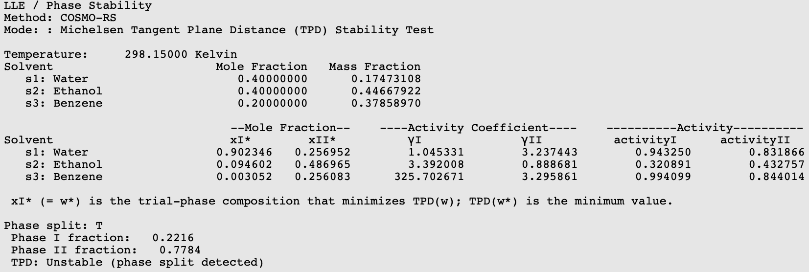
The tangent plane distance (TPD) phase-stability test checks whether a given feed composition remains a single liquid phase or is expected to split into two liquid phases.
In this example, we use the ternary system water (1) + ethanol (2) + benzene (3).
TPD STABILITY Test3 componentsMole fraction0.40.40.2298.15 and unit = KRun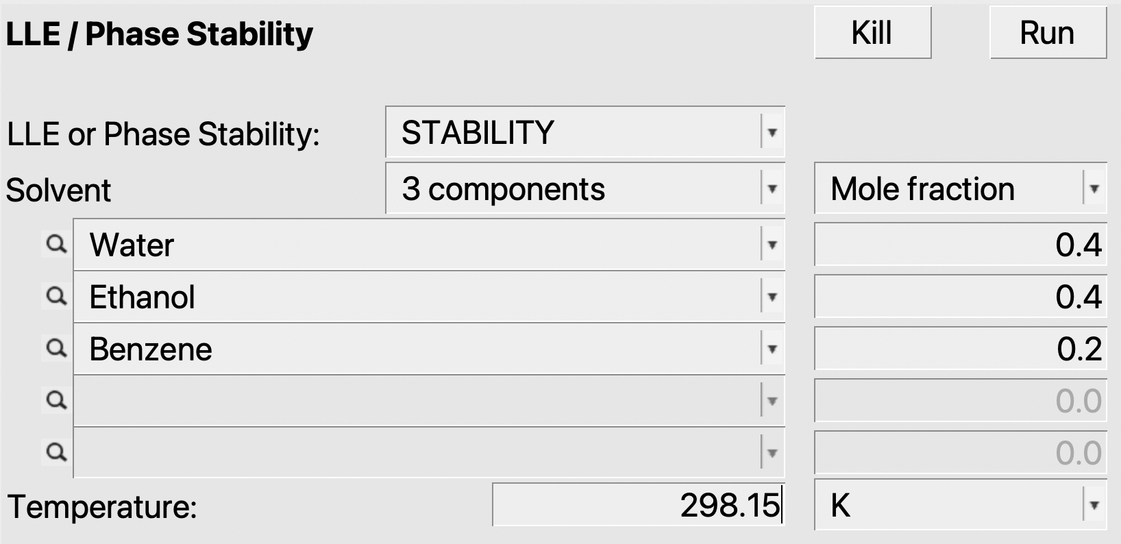
If phase splitting is detected, \(x_I^*\) is the resulting trial-phase composition. The corresponding \(x_{II}^*\) and phase fraction are back-calculated from the feed composition by material balance, i.e., \(z = (1-L)\,x_I^* + L\,x_{II}^*\). Although it may still be far from the equilibrium composition, it provides a useful initial guess and is used by default as a built-in initialization for the LLE solver.
If the ethanol fraction is increased, the mixture is reported as stable (no phase split detected), for example:
0.20.60.2Liquid-Liquid Equilibrium
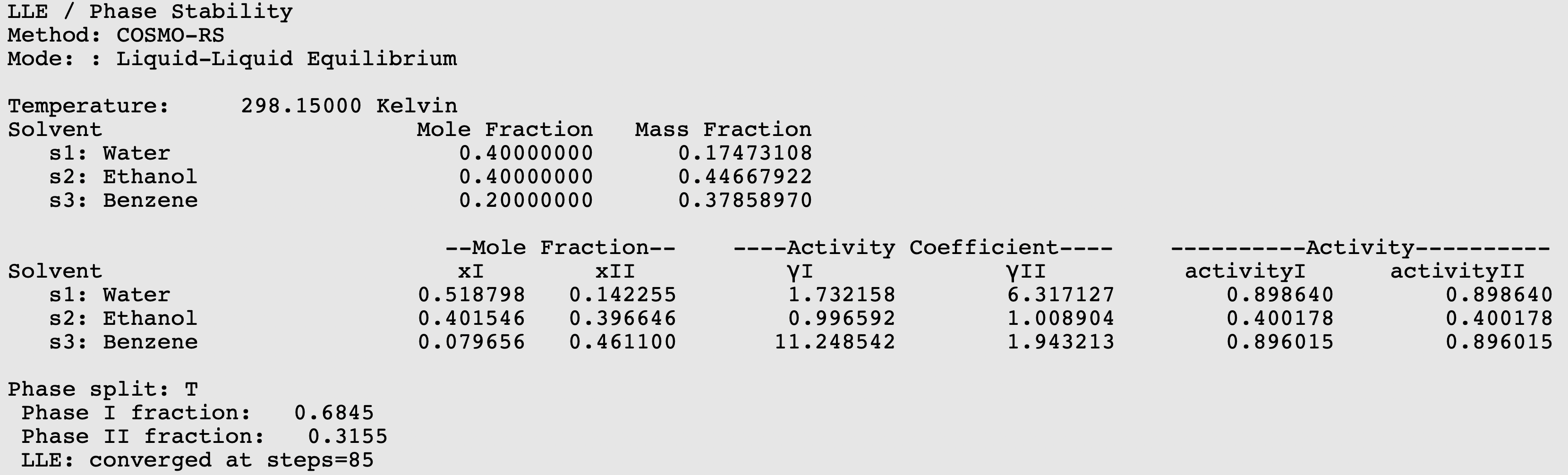
Here, we switch to an LLE calculation for water (1) + ethanol (2) + benzene (3).
LLE0.40.40.2When phase splitting is detected in the build-in stability test, the LLE solver searches for a two-liquid-phase equilibrium that satisfies equality of component activities between the two liquid phases. The current algorithm considers only two liquid phases at equilibrium.
The LLE output reports mole fractions, activity coefficients, and activities for the two equilibrium liquid phases.
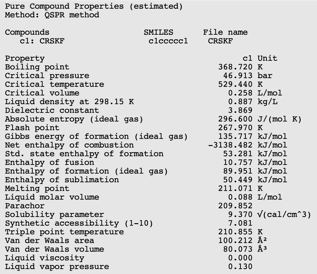
Step 12: Pure Compound Properties
A QSPR (Quantitative Structure-Property Relationship) method can be used to estimate some pure compound properties. This QSPR method needs a SMILES string as input.
Openbabel is used to generate a SMILES string for benzene, which should be “c1ccccc1”.
Step 13: Solvent Optimizations: Optimize Solubility
Note that the solvent optimization code has fixed parameters for COSMO-RS: the AMS combi2005 parameter set with the f_corr parameter set to 0.
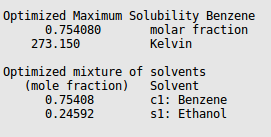
In this step a solvent is optimized in order to maximize or minimize the mole fraction solubility of a solid solute in the liquid mixture. A list of pure solvents should be provided. The optimal solution might be one of the pure solvents, but might also be a mixture of these solvents. Note that if the optimal solution is a mixture of solvents, no check is done whether these solvents are in fact miscible. Note that for the solubility of a solid compound it is necessary to include the melting point and the enthalpy of fusion of the solid. First we try to optimize the solvents, such that it maximizes the solubility (mole fraction) of solid benzene
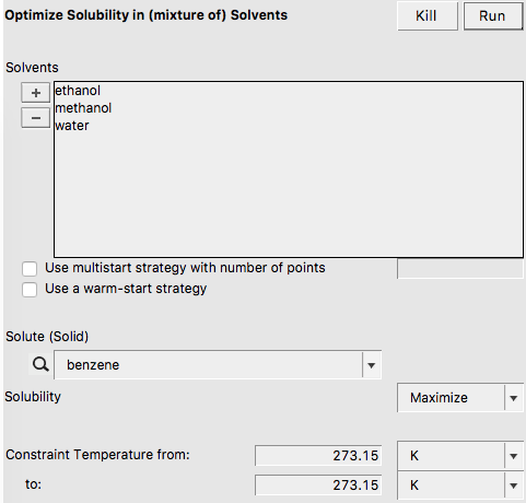
In this case the pure solvent ethanol is found as optimal solvent
Next we try to optimize the solvents, such that it minimizes the solubility (mole fraction) of solid benzene
In this case, the pure solvent water is found as optimal solvent.
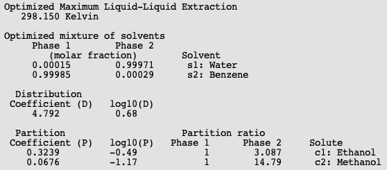
Step 14: Solvent Optimizations: Optimize Liquid-Liquid Extraction
Note that the solvent optimization code has fixed parameters for COSMO-RS: the AMS combi2005 parameter set with the f_corr parameter set to 0.
In this step a mixture of immiscible solvents is optimized in order to maximize or minimize the distribution ratio (D) of two solutes between the two liquid phases. A list of pure solvents should be provided. At least two of these solvent should be immiscible with each other. In this example we try to optimize the mixture of immiscible solvents for liquid-liquid extraction (LLE) of methanol and ethanol.
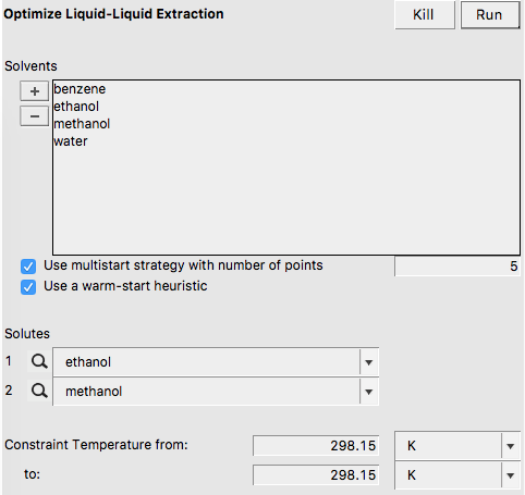
In this case the optimized mixture of immiscible solvents is benzene and water.