Caffeine Bader (AIM) analysis, Benzene NBO visualization and Occupations¶

Step 1: Setup and optimize Caffeine¶

Start ADFinput

Next we need a reasonable guess for the structure of Caffeine. The quickest way to do this is to search for it in the database of molecules included with the ADF-GUI, and optimize it:

Press cmd-F or ctrl-F to activate the search box

Type ‘caffeine’ in the search box

Move your mouse pointer on top of the ‘Thein’ search result

As you can see, there are several matches. If you position your mouse over the results (without clicking) a balloon will appear showing the details of that match. For this tutorial we use the second match “Thein”, from the NCI database. Thein is one of the common names for caffeine (and as you can see there are may alternative names),

Click on the ‘Thein’ search result

Click somewhere in empty space in the molecule drawing area to deselect the atoms

Switch to DFTB mode (panel bar ADF → DFTB)

Select model: SCC-DFTB

Make sure the parameter set is “Dresden” (normally you would want to use better parameters like the included 3OB set)

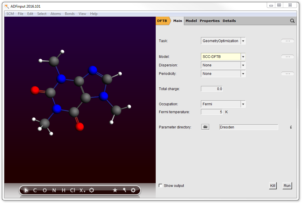
Note that only those parameter sets known to be able to handle your system will be shown in the menu.

If you move your mouse over the parameter field, the information balloon will also show references applicable to the selected set of DFTB parameters. More detailed information and references will be displayed if you click on the ‘i’ button next to the parameter input field.

Click the ‘Run’ button

If the message says ‘NOT converged’, press ‘Run’ again.

The DFTB program should have created something similar to this structure:

Step 2: Calculation setup¶

Next we will calculate the AIM critical points and paths for the current structure.

Switch to ADF mode (panel bar DFTB → ADF)

Now we want to activate the Bader AIM analysis to find the critical points and bond paths. To find where this option is located, search for it:

Activate the search box (cmd/ctrl-F)

Type ‘criti’ in the search box

Use the Return key to accept the highlighted match (Other...)

ADFinput will activate the panel that displays the option you are looking for (to calculate the AIM critical points and paths). The matching input options will be marked with blue italic text. Note that we first had to activate the ADF mode, the input option search will restrict the search to panels that belong to the current method (ADF, BAND, DFTB, ...)

Check the box to calculate Bader (AIM ) Critical points, bond paths and atomic properties

Check the box to calculate AIM atomic energies

Check the box to save the Bader basins

Run this setup: File → Run

A dialog will pop up in which you must specify a filename to use for your job, for example caffeine:

Enter ‘caffeine’ as a Filename, press the Save button

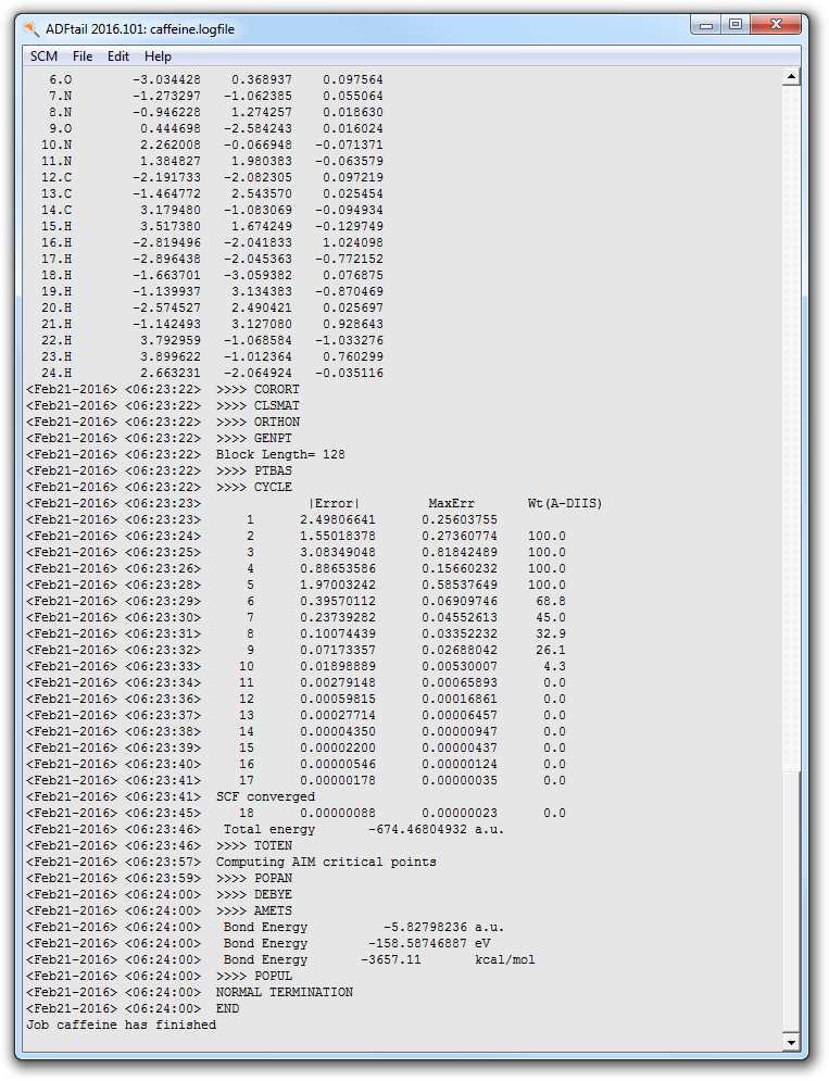
After hitting the save button the calculation will start. You will get two extra windows: first a window for ADFjobs that allows you to manage your jobs and keep track of their state (for example, queued or running). You will also get a window showing the ADF log file. This shows you what is going on in the current calculation.

Depending on your computer, the calculation should be ready after a few minutes at most:

Step 3: Orbitals, Potential and AIM results¶

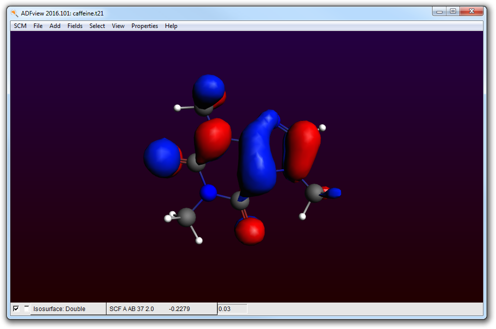
Start ADFview SCM → View

Show the HOMO Properties → HOMO

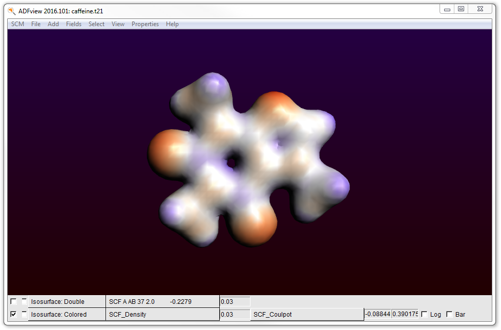
Hide the HOMO by unchecking the check box at the lower left corner of the ADFview window

Add → Isosurface: Colored

In the first field selector (to the right of the ‘Isosurface: Colored’ text at the bottom), select Density → SCF

In the second field selector (to the right of the ‘0.03’ text in the same line), select Potential → SCF

Hide the surface with the potential energy: uncheck the check box at the lower left corner of the window

Properties → AIM (Bader)

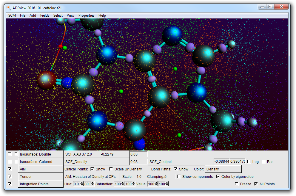
The critical points and bond paths are shown (the molecule balls and sticks representation is hidden). The different types of critical points (atom CP, bond CP, ring CP and cage CP) are indicated by different colors. The atom CPs are scaled by density by default, which makes them look like atoms. The bond paths are colored by density, by default.

You can also visualize the Hessian of the Density in the critical points:

Uncheck the ‘Scale By Density’ check box in the AIM line at the bottom of the window

Properties → AIM: Hessian of Density at CPs

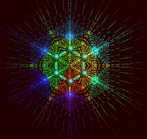
To get a rough display of the Bader basins, use the Bader sampling option:

Properties → Bader Sampling

Zoom in

The different colored points show the different basins.

ADFview has many options to visualize the results, the options just used are mainly to show off some features. Play around with the different options, for example try out what the check boxes do on the left side. Or try other fields, or colored cut planes, or ...

This finishes the Caffeine Bader (AIM) tutorial, close all its windows:

SCM → Quit

Step 4: Benzene Bader charge analysis and NBOs¶

Start ADFinput

Make a benzene molecule (for example by searching for it with cmd/ctrl-F)

Set up a Single Point calculation without frozen cores

Panel bar Properties → Other: Etot, Bader, Charge Transport, ...

Check the ‘Atomic energies’ option

Check the ‘Save Bader atomic basins’ option

Panel bar Properties → Localized Orbitals, NBO

Check the ‘Perform NBO analysis’ option

Request Boys-Foster localized orbitals

Run this setup (File → Run)

When the calculation is done (it should run very fast), we use ADFview to examine the Bader charges and compare them with Mulliken charges:

Open the results with ADFview

Show the Bader atomic charges (Properties → Atom Info → Bader Charge → Show)

Color the atoms by Bader charges (Properties → Color Atoms By → Bader Charge)

Show the Mulliken charges (Properties → Atom Info → Mulliken Charge → Show)

Next we inspect the NBOs and Boys-Foster localized orbitals. To remove the charge display we close and open ADFview, but you could also have used the View menu to remove them by hand:

Close ADFview

Open the results again with ADFview

Add a Double Isosurface

Use the field menu in the new control line,

and observe the labels present with the NBOs and NLMOs

Open NBO number 15 (should be similar to C6-H12)

Improve the grid by using Fields → Grid → Fine

Obviously, you can also visualize the NLMOs or the Boys-Foster localized orbitals (which are just called Localized Orbitals in the fields menu.

Next we inspect the Bader atomic basins. The numerical integration points are used for this purpose. The color indicates to which atomic basin the numerical integration point belongs to.

Close ADFview

Open the results again with ADFview

Properties → Bader Sampling

One can also select one or more atoms, to see only the Bader atomic basins of the selected atoms.

Step 5: Occupations¶

Now we will remove one electron from a selected orbital (by symmetry) using ADFinput again.

Open your benzene calculation in ADFinput

Model → Spin and Occupation

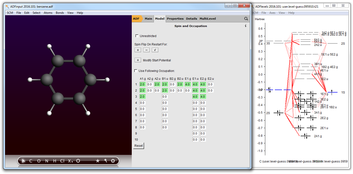
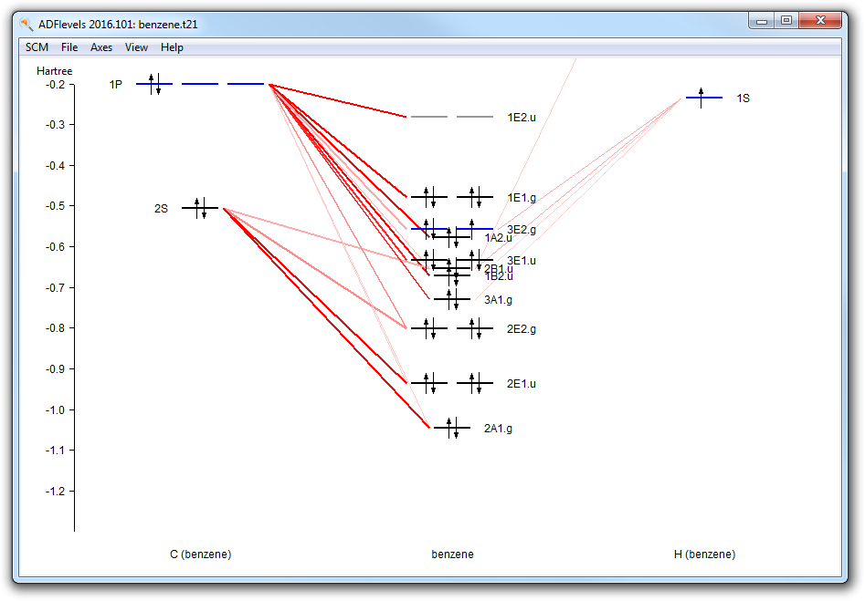
In the Spin and Occupation panel you see which orbitals are available (by symmetry, and spin if the current set up is unrestricted). The numbers are the occupations. Next to the ADFinput window ADFlevels will also have opened, and is showing a level diagram of your current molecule. This helps you to select the proper occupation.

The level diagram is based on the existing result file (.t21) found. If none, ADFinput will suggest to do a guess-calculation: a hopefully fast calculation using an inaccurate integration grid, and stopping after a few SCF cycles. The level diagram shown in that case will not be accurate obviously but will still be helpful in selecting the proper occupation.

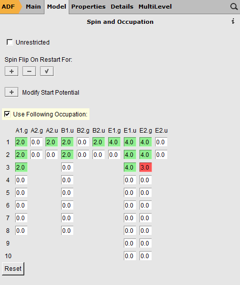
Now, just as an example, we make a hole in the 3E2.g orbital. Note that this is NOT the HOMO.

Change the 4.0 to 3.0 in the 3 E2.g column (the third row)

Close the guess adflevels

File → Save

Close the ADFinput window

Run (via the Job → Run command in ADFjobs

When the run is complete:

Open ADFlevels using the SCM → Levels command

In the ADFlevels window, use the View → Labels → Show command

Zoom in to the region of interest (for example using your mouse wheel)

In the levels diagram you will observe that the HOMO (the 1E1.g) is completely filled, while the orbital below it has a hole. You can easily see this by the color. Note that we have performed a restricted calculation, so in effect the hole is averaged over the E orbitals.