Excitation energies and UV/Vis spectrum of ethene
First you will construct an ethene molecule and optimize its geometry. As this is basically the same procedure as in Tutorial 1, only short instructions will be given.
Next you will set up the calculation of excitation energies, and let ADF perform the calculation.
Finally, using ADFlevels, ADFspectra and ADFview, you will examine the results.
Step 1: Start ADFinput
For this tutorial we again prefer to work in the Tutorial directory.
You know how to start ADFjobs (in your home directory), and move to the Tutorial directory:
- cd $HOMEStart ADFjobsClick on the Tutorial folder icon
Next start ADFinput using the SCM menu:
- Select the SCM → New Input command
Note that if you start ADFinput via the SCM menu you will start ADFinput without loading a job. If you wish to open ADFinput for a particular job, click on the ‘ADF’ button in front of it.
For the View command (and Movie, Levels, and so on) the behavior is different: it will immediately load the job that is selected in ADFjobs.
Step 2: Create your ethene molecule
First we construct an ethene molecule, and pre-optimize its geometry:
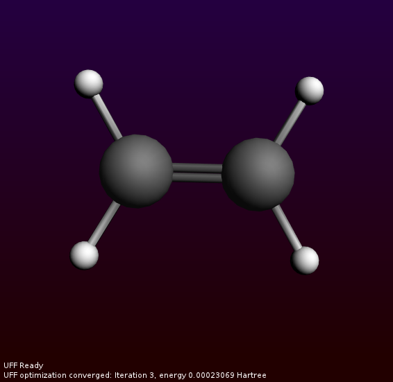
- Select the C-tool by clicking on the button with the ‘C’Select the Double bond mode Bond tool → Double(or use the shortcut: press the ‘2’ - key)Click somewhere in the drawing area to create a carbon atomClick again to create a second carbon atom (with a double bond)Click on the just created Carbon atom to stop bondingSelect the Atoms → Add Hydrogen commandClick the cog wheel to pre-optimize
Your ethene molecule should look something like this:
Step 3: Optimize the geometry
The next step is to optimize the geometry using ADF:
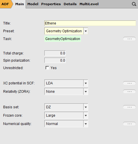
- Enter a title in the Title field (like ‘Ethene’)Select the ‘Geometry Optimization’ preset
With the proper options selected, now run ADF:
- Select the File → Run commandClick ‘Yes’ in the pop-up to save the current inputIn the file select box, choose a name for your file(for example ‘ethene’) and click ‘Save’
Now ADF will start automatically, and you can follow the calculation using the logfile that is automatically shown.
- Wait until the optimization is ready (should take very little time)
The following dialog should appear:
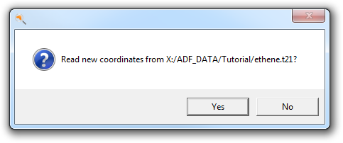
- Click ‘Yes’ to update the coordinates
Step 4: Calculate the excitation energies
Select calculations options
To set up the calculation of the excitation spectrum:
- Adjust the title to something like ‘Ethene excitations’Select the ‘Single Point’ presetUse the panel bar Properties → Excitations (UV/Vis), CD command to go to the Excitations panelFor the ‘Type of excitations’ option, Select ‘Singlet and Triplet’
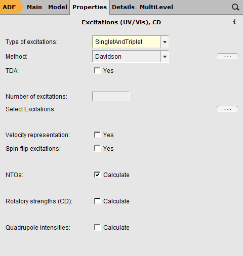
For the tutorial this set up is fine, normally you would also need to select an XC potential that gives better results, for example SAOP.
Run the calculation
Now everything is ready to actually run ADF. Before running we will save the current input in a different file (though this is not really required):
- Select File → Save As...Enter a filename (ethene-exci) and click ‘Save’Select File → RunWait for the calculation to finish
Step 5: Results of your calculation
Logfile: ADFtail
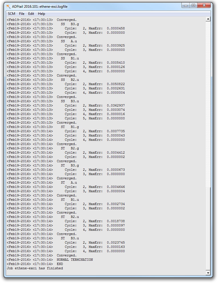
The logfile shows you that the calculation has finished, and that indeed the excitation code has been running:
- Select SCM → Logfile
Energy levels: level diagram and DOS
- Select SCM → Levels
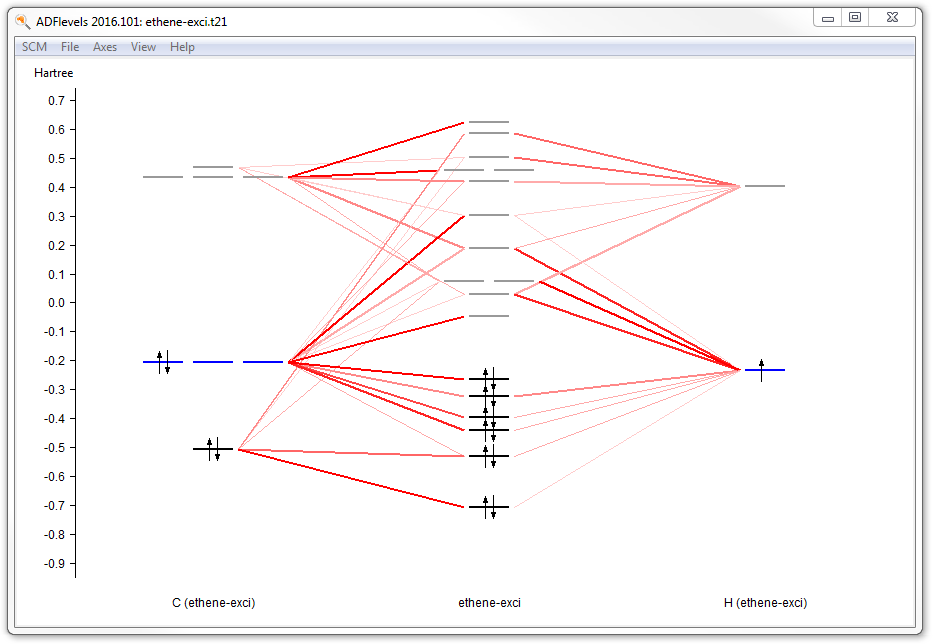
In this level diagram you can see that the HOMO and LUMO consist mainly of carbon p orbitals. It is also easy to see what orbitals the hydrogens take part in.
Note that the carbon and hydrogen stacks show all carbon and hydrogen atoms at once: they show the fragment type. ADFlevels can also show the individual fragments but when using atomic fragments you will get too many fragments. In this particular case symmetry is used, and since there is only one symmetry unique carbon atom and only one symmetry unique hydrogen atom you still would see only one stack per atom type.
- Select SCM → DOSIn the ADFdos window:View → Add GraphSelect one hydrogen atom
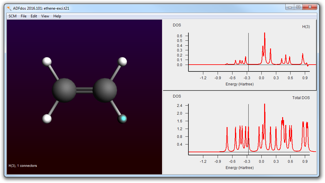
In these plots you can see that the partial DOS for the hydrogen atoms have no contribution to the HOMO. By right clicking on an atom you can also show partial DOS graphs with contribution from selected atoms and selected L-values only.
Excitation spectrum: ADFspectra
- Select SCM → Spectra
ADFspectra will start and show the calculated excitation spectrum.
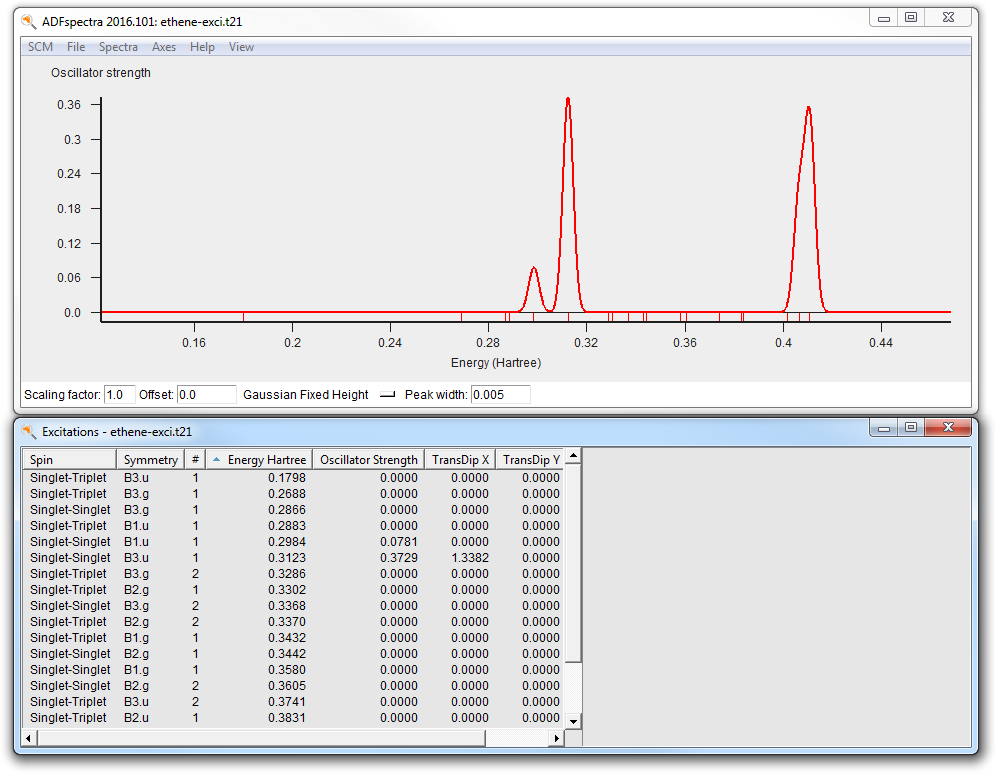
In the window below the spectrum you will find a table with information. You can get more information by selecting one of the entries (or click on the peak in the spectrum):
- In the table select the Singlet-Singlet1B3.u peak
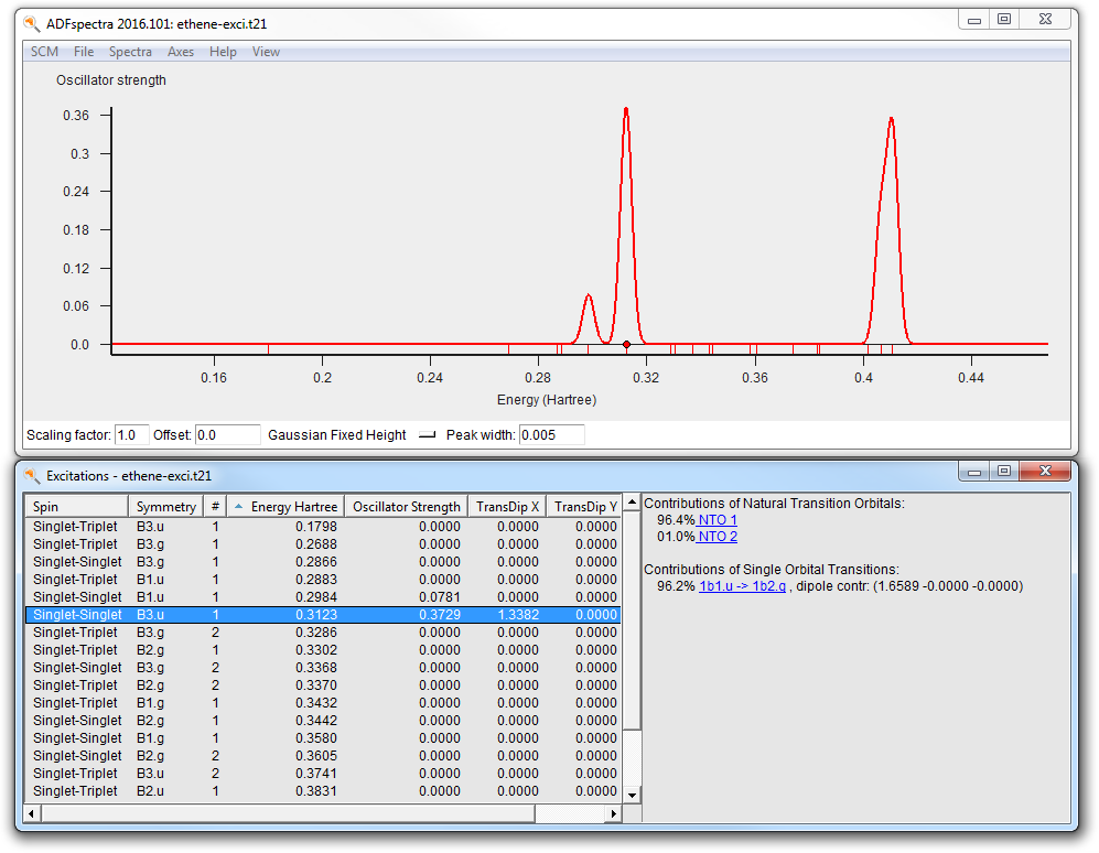
The composition of the excitation in terms of orbital transitions is listed on the right side. In many cases you can visualize relevant orbitals or NTOs with ADFview by clicking on them in the window on the right. The clickable items are visually marked.
- Click on the the first major contribution line (with the highlighted orbitals)
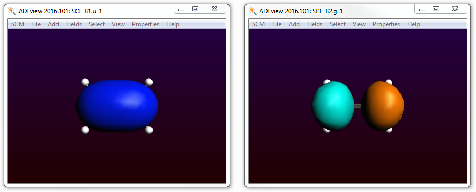
- Close the two windows showing the orbitals using File → Close in both windows
Orbitals, orbital selection panel: ADFview
We will now use ADFview to examine the orbitals. Not just one, but have a look at many of them. To do that ADFview has an ‘orbital selection’ panel.
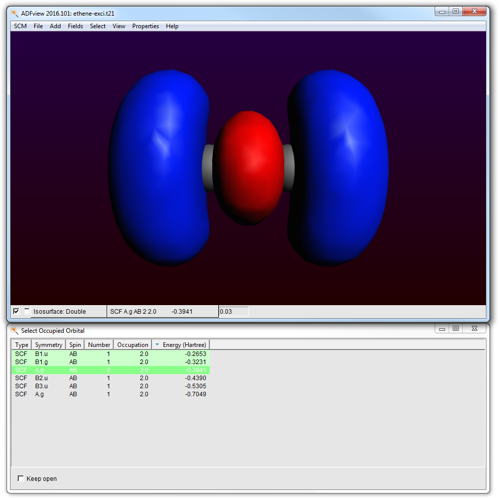
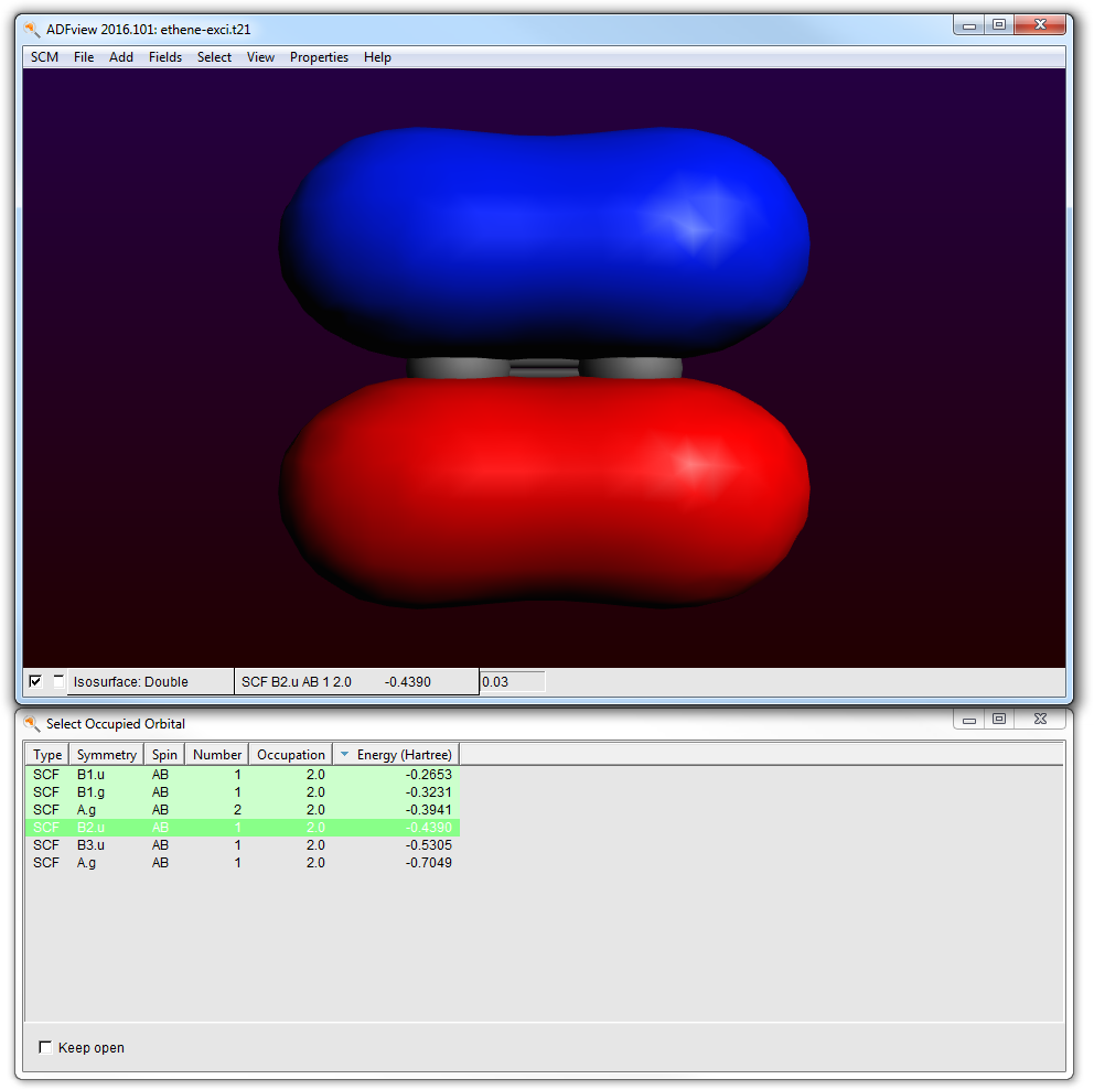
- Select SCM → ViewSelect Properties → HOMOClick on the field selector pull-down in the control bar for the HOMO (reading SCF_B1.u 1: ...),select Orbitals (occupied)
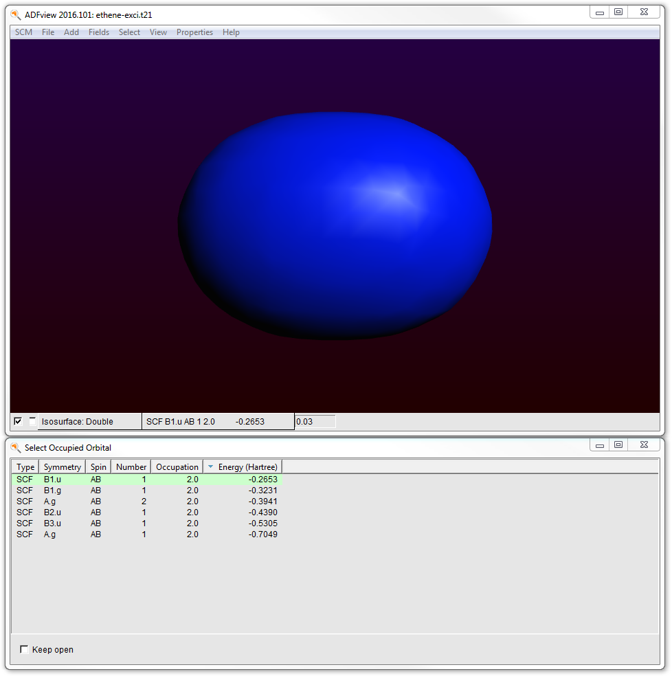
In the ‘Select Occupied Orbital’ window you can select the orbital that you want to see. Note that the currently visible orbital is highlighted using a dark green background.
- Click on all of the orbitals in the window, one by one, and observe the orbitalsClick again on them
When you click the first time on an orbital, its values need to be calculated and then the orbital is shown. When you click for a second time on an orbital in the list, it has already been calculated (indicated by the light green background color). And thus it shows immediately.
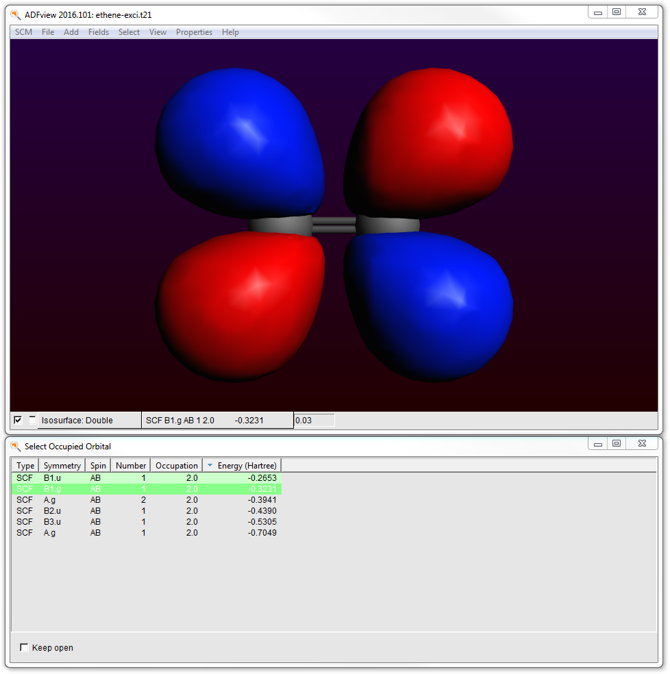
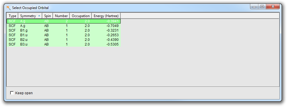
The Orbital select window allows you to reorder the orbitals by clicking on the headers of the columns. Thus you can sort by Symmetry, Spin, etc. Clicking again on a header reverts the sort order.
- Click on ‘Symmetry’ in the ‘Select Occupied Orbital’ window
- Close ADFview: File → Close
Transition density: ADFview
You can use ADFview to view orbitals etc, but also to have a look at the transition density.
- Select Add → Isosurface: Double (+/-)
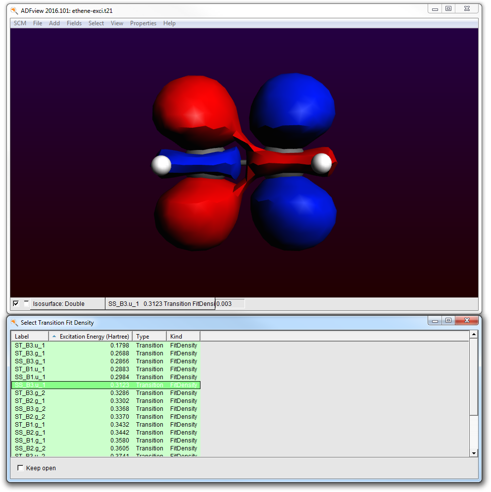
In the field pull-down menu (in the control line for the double isosurface) you will find an entry ‘Transition Density’, and if you select it an orbital select box will shown with all available transition densities:
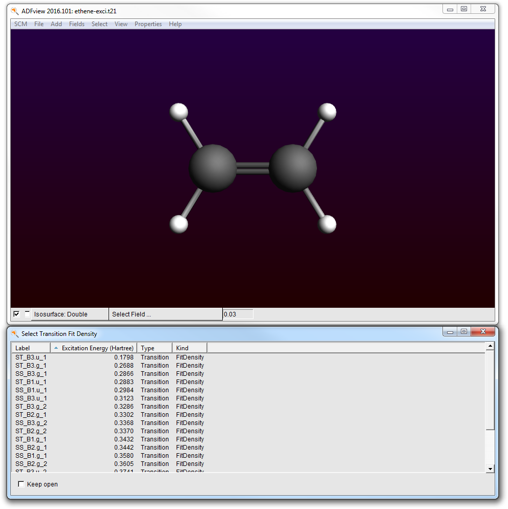
In this case lets select the transition density that belongs to the biggest peak: the Singlet-Singlet 1B3u excitation:
- Click on the TransDens_SS_B3.u_Fitdensity_1 fieldChange the iso value to 0.003Rotate the molecule a little
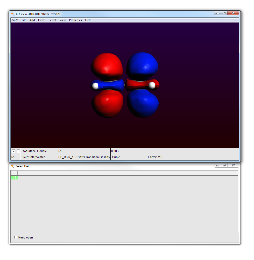
The resolution is rather coarse, you can use interpolation to get a better picture.
- Fields → InterpolatedSelect the Transition Density → TransDens_SS_B3.u_Fitdensity_1 field in the I-1 lineIn the Isosurface: Double line, change the field to I-1 (in the Other category in the field selector)
ADF Output
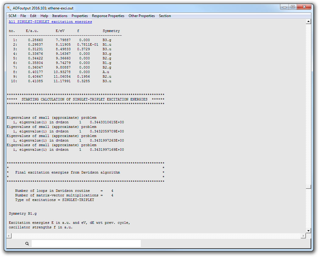
Using the output browser you can find all details about your excitation calculation. Use the menu to jump to the relevant part of output:
- Select SCM → OutputSelect Response Properties → All Singlet-Singlet Excitation Energies
KFBrowser
Most result of the calculation are saved to the KF result file (the .t21 file for an ADF calculation). You can inspect the contents of KF files using the KFBrowser. The KFBrowser is a very recent development, feedback and bug reports (there will be bugs...) are welcome!
The KFBrowser gets the raw data out of the result file, and presents a selection of that might be of interest for users. Over time more results will probably be added to newer versions of the KFBrowser.
It also gives access to all raw data in the result files. This feature is intended for developers only.
- Select SCM → KFBrowserIn the KFBrowser window that appears:Click on the arrow in front of ExcitationsClick on the arrow in front of Energies (Hartree) (in the Excitations section)

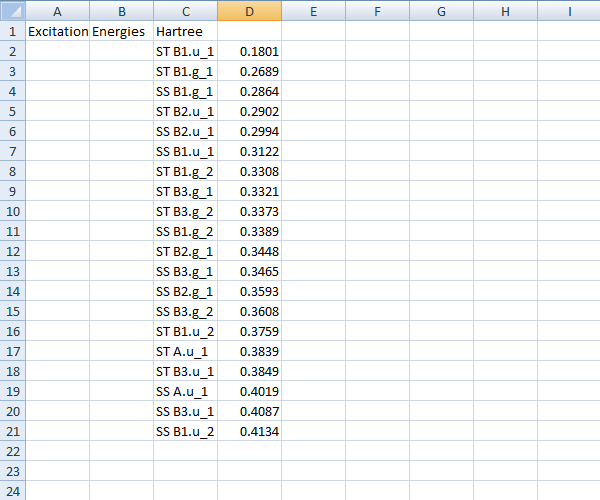
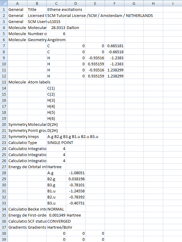
If you click on the name of the property you can select it. Next you can copy it, and paste it for example in Excel:
- Click on “Energies (Hartree)”Copy (from the Edit menu or the usual shortcut)Open Excel or some text editorPaste
After pasting you should have your results nicely formatted in Excel or in some text document. Note that the values are tab-separated, so pasting into Excel will automatically put the data (energies) in cells.
In a similar way you can copy/paste other results. Or even all results:
- In the KFBrowser window:Edit → Select AllEdit → CopyIn the Excel or text editor window:Paste
All results should be nicely formatted in your text document or spreadsheet:
Another feature of the KFBrowser is that it can show results in simple graphs:
- Close the KFBrowser windowOpen it again SCM → KFBrowserOpen the Charges sectionClick on Mulliken (e)Shift-click on MDC-Q (e)Use the Graph → Selection As Graph command (or double click on the selection)
A window should appear that shows the selected results, charges in this case:
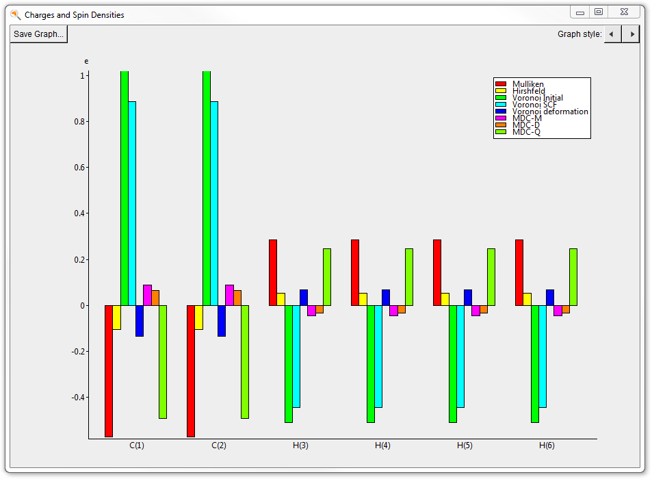
You can use the Graph style buttons to switch to different graph types (XY, Bars or Piechart).
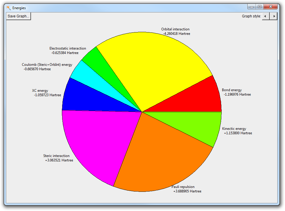
- Switch to the KFBrowser windowOpen the Energies sectionSelect all energies (click on first, shift-click on last energy)Double click on the selection
Finally two features that are intended for developers and expert users: the KFBrowser module can also show the raw data on the result file, and it can dump a KF file as a plain text file. To activate the expert mode, use the File → Expert Mode menu command. To save the contents of the result file as a text file using the File → Save As ASCII... command.
Step 6: Excited state geometry optimization and excited state density
With ADF you can also optimize the geometry of some selected excited state. It depends on your application which state to optimize, in this tutorial we will pick the state corresponding to the largest peak in the UV/Vis spectrum.
- Determine the name of the excited state corresponding with the largest peak in ADFspectra (1B3.u)If your molecule has a different symmetry the name may be different!In ADFjobs: click on the ADF button in front of the ethene-exci job
ADFInput should open with the ethene-exci job (or come to the front if already open).
- Select the Geometry Optimization presetSelect Frozen Core: NoneOpen the Excited State Geometry panel in the Properties menuEnter the excited state to optimize (1B3.u)File → Save As...Save the file with a name like ‘ethene-exci-1B3u’File → Run
With ADFmovie you can see how the excited state geometry is different from the ground state geometry:
- Wait for the calculation to finishSCM → MovieObserve how the geometry changes
With ADFmovie you can see how the excited state density is different from the ground state density:
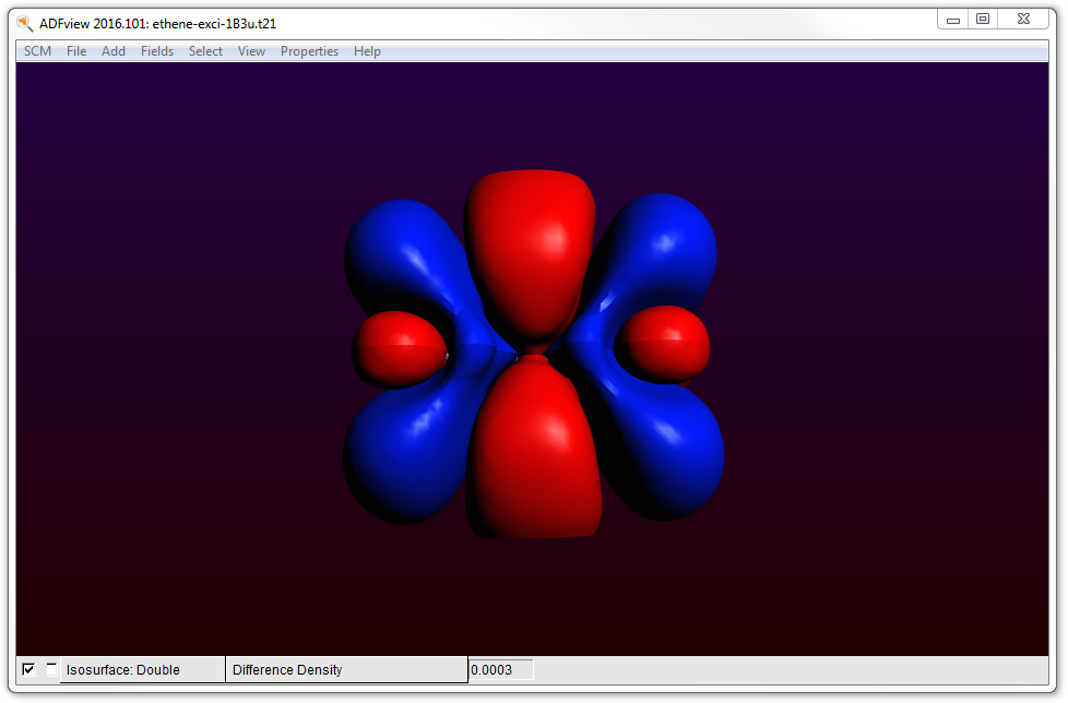
- SCM → ViewAdd → Isosurface: Double (+/-)In the field select menu on the bottom: select Excited State → Difference DensityChange the isovalue to 0.0003Fields → Grid → Medium to get a better quality
Now you see how the excited state density differs from the ground state density (for this geometry)
If you wish to see the excited state density, you can do this using a Calculated field (add the ground state density to the difference density).
Closing the ADF-GUI modules
To close all modules for your excitations calculation at once, use the Close command from the SCM menu:
- Select SCM → Quit
Close will close all open modules that have your current job loaded, except ADFjobs. The Close All command will close every ADF-GUI module, including ADFjobs:
- Select SCM → Quit All
All ADF-GUI modules (and BAND-GUI modules if any) should be closed.