Getting started: Geometry optimization of ethanol¶

Start ADFjobs¶

On a Unix-like system, enter the following command:

cd

adfjobs &

On Windows, one can start ADFjobs by double-clicking on the ADF-GUI icon on the Desktop:

Double click the ADF-GUI icon on the Desktop

On Macintosh, use the ADF2016.xxx program to start ADFjobs:

Double click on the ADF2016.xxx icon

Make sure X11 allows you to use keyboard shortcuts (you only need to do this once):

Press Cmd-,

If nothing happens everything is fine.

If the X11 Preferences dialog appears:

uncheck the “Enable key equivalents under X11” check box and close that dialog.

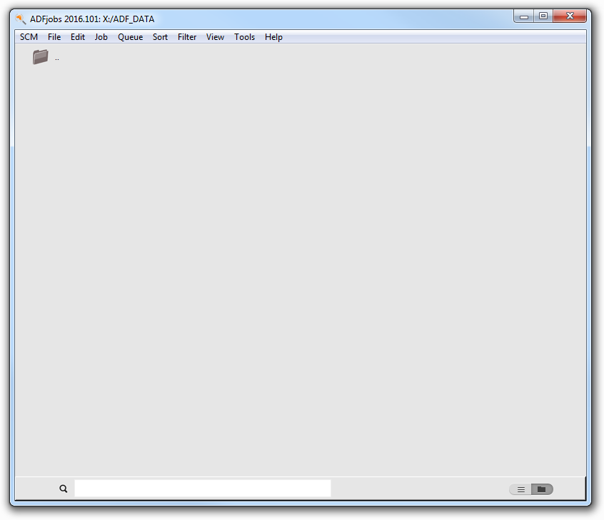
Note that the directory in which ADFjobs depends on how you start ADFjobs, so your screen might look different.

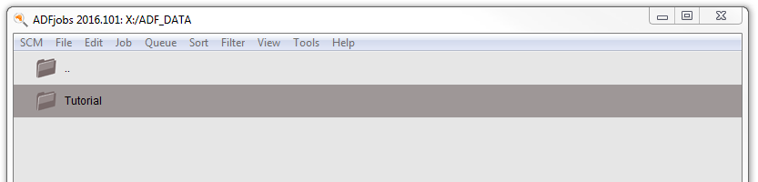
Make a directory for the tutorial¶

We prefer to run the tutorial in a new, clean, directory. That way we will not interfere with other projects. ADFjobs not only manages your jobs, but also has some file management options. In this case we use ADFjobs to make the new directory:

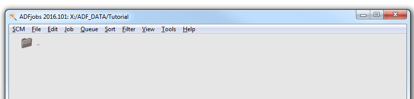
Select the File → New Directory command (thus, the New Directory command from the File menu)

Rename the new directory by typing ‘Tutorial’ and a Return

Change into that directory by clicking once on the folder icon in front of it

Start ADFinput¶

Now we will start ADFinput in this directory using the SCM menu:

Select the SCM → New Input menu command:

use the SCM menu on the top left (the SCM logo on most platforms),

next select the New Input command from the menu.

The ADFinput module should start:

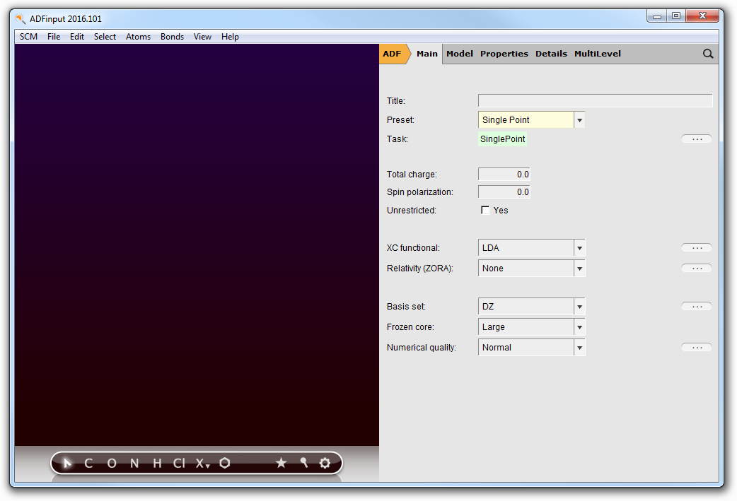
The ADFinput window consists of the following main parts:

• the menu bar with the menu commands (File, Edit, ...)
• the drawing area of the molecule editor (the dark area on the middle left side)
• the status field (lower part of the dark area, blank when the ADFinput is empty as shown above)
• the molecule editor tools
• many panels with several kinds of options (currently the ‘ADF Main’ panel is visible)
• panel bar with menu commands to activate the panel of choice
• a search tool (at the right of the panel bar)

Undo¶

ADFinput has an Undo command, which works on your molecule (thus not on your input options).

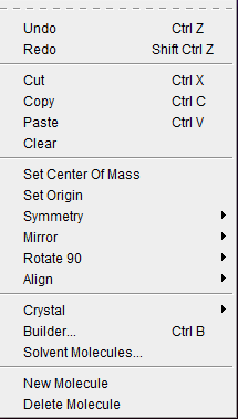
If you make a mistake while making changes to your molecule, just use the Edit → Undo menu command to go back in time.You can Undo more than one step, or Redo a step (with Edit → Redo) if you wish to do so.

Create a molecule¶

The molecule we are going to create is ethanol.

First we will draw the two carbon atoms, next the oxygen atom, and after that we will add all hydrogen atoms at once. Finally, we will pre-optimize the geometry within ADFinput.

Create the first carbon atom¶

To create an atom, you need to select an atom tool.

Select the C-tool by clicking on the button with the ‘C’

Back glow is added to the ‘C’ button to indicate that you are using the C-tool. Also, the status field in the left bottom corner shows ‘C tool, create single bond’ to indicate that you are using the C-tool.

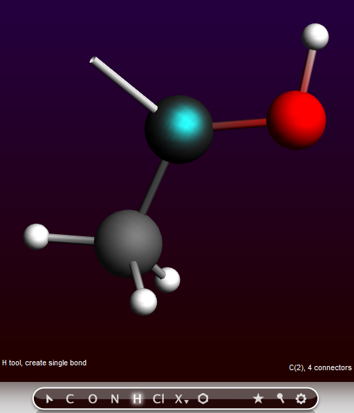
Now create the first carbon atom:

Click somewhere in the drawing area

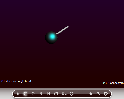
One carbon atom has been created.

Note that:

• If you move the mouse you will see a white line from that carbon atom to the current mouse pointer position: this shows you are in ‘bonding’ mode, and that the bond will be made to the atom just created.
• The ‘C’ button has a different color, indicating you are still using the C-tool.
• The carbon atom is selected (the green glow), which indicates that the carbon atom is the current selection.
• The status field contains information about the current selection: it is a Carbon, number 1, with 4 ‘connectors’
• The status field also shows the current tool (C), and that a single bond will be made.

Create the second carbon atom¶

Click somewhere in the drawing area to create the second carbon atom

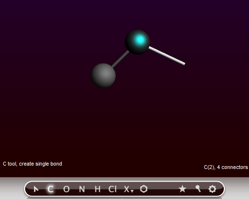
A second carbon atom has been created, bonded to the first atom.

The atom will be created along the ‘bonding line’, at a distance that corresponds to a normal C-C single bond distance. That is, the bond length is constrained while drawing.

The newly created atom becomes the new selection, and you are still in bonding mode. The next bond will be created to the carbon atom just created. And you are still using the C-tool.

Create the oxygen atom¶

To create the oxygen atom you need to switch to the O-tool:

Select the O-tool by clicking on the button with the ‘O’

With the O-tool, create an oxygen atom bonded to the second carbon;

Click somewhere in the drawing area

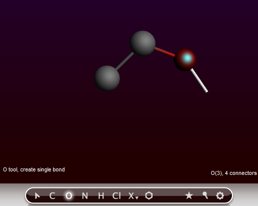
The oxygen atom has been added.

For now, we are done using atom tools, so go back to the select tool:

Select the select-tool by clicking on the button with the arrow (or press the Esc key)

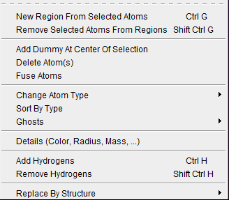
Add the hydrogens¶

Now many hydrogen atoms need to be added. You can do this using the H-tool, but a much easier method is to use the Atoms → Add Hydrogen menu command:

The ‘Add Hydrogen’ menu command works on the selection only, when present. Thus, only one hydrogen atom would be added to the oxygen atom. This is not what you want. So first we make sure that nothing is selected by clicking in empty space.

Click in empty (drawing) space

Now no atoms are selected any more.

Select the Atoms → Add Hydrogen command

Many menu commands have shortcuts. In this case you can also use the shortcut (ctrl-H or cmd-H, depending on your platform) as an alternative. The shortcuts are indicated in the menu commands.

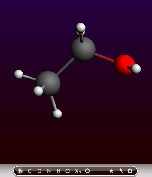
All atoms will be saturated with hydrogen atoms. And you have created an ethanol molecule, though the geometry is still far from perfect.

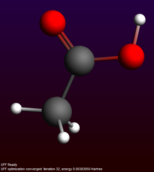
Pre-optimize the geometry¶

Now use the optimizer that comes with ADFinput to pre-optimize the geometry.

Click on the pre-optimizer button (the rightmost ‘cog wheel’ button of the menu bar)

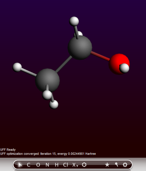
The geometry of the molecule will be pre-optimized, using UFF by default. Note you can select another pre-optimizer via the Preferences, or use a different pre-optimizer by right-clicking on the cog wheel and selecting the method to use from the pop-up menu.

In the status field below the drawing area you can follow the pre-optimization iteration number and the energy relatively to the starting configuration.

Viewing the molecule¶

Rotate, translate, or zoom¶

You can rotate, translate, and zoom your molecule using the mouse.

You need to drag with the mouse: press a mouse button, and while holding it down move it. Which mouse button, and which modifier key you press at the same time, determines what will happen:

Rotate	Left
Rotate in-plane	ctrl-Left
Translate	Right
Zoom	Mouse wheel, or alt-Left (drag up or down)

The rotate, translate, and zoom operations change how you look at the molecule, they do not change the coordinates.

This behavior is the default behavior, you can change what the right mouse button does using the Preferences.

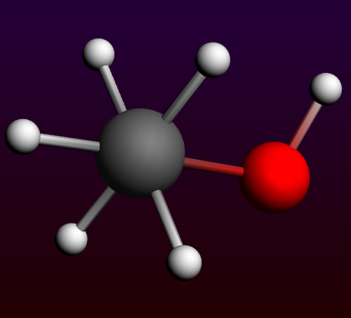
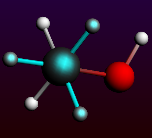
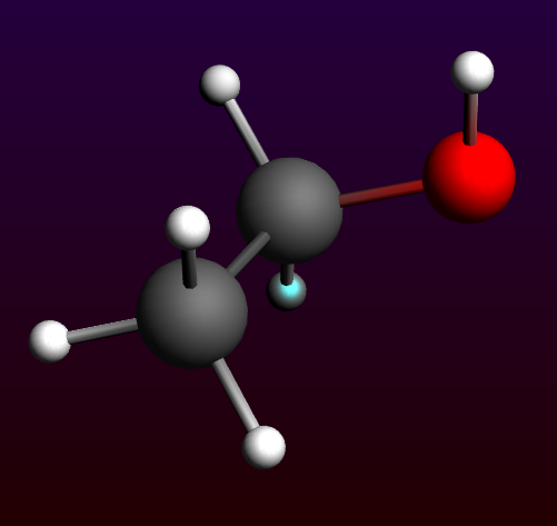
Click once somewhere in empty space to make sure nothing is selected.

Click with the left mouse button, and drag:

your molecule will rotate.

Click with the left mouse button with the ctrl-key, and drag:

your molecule will rotate in-plane.

Click with the right mouse button, and drag:

your molecule will be translated.

Click with the right Middle button (if available), and drag up and down:

you will zoom closer to or away from your molecule.

Click with the left mouse button with the alt-key, and drag:

you will zoom closer to or away from your molecule.

Use the mouse wheel, if you have one:

you will zoom closer to or away from your molecule.

Using all these options, try to position the ethanol as in the following image:

Save picture¶

You can save a picture of your molecule using the ‘Save Picture ...’ command from the File menu.

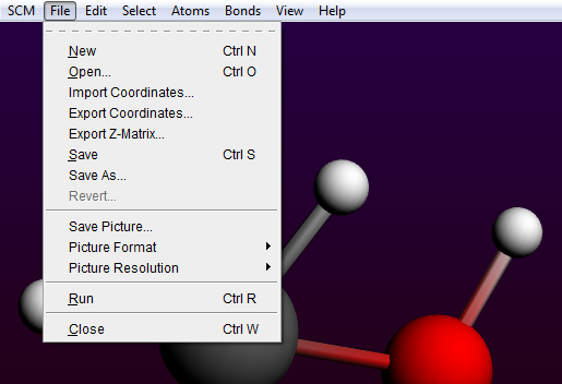
The format used is the PNG format. You can change this using the File → Picture Format menu command. You can also change the resolution. A smaller resolution will result in a smaller file, but will reduce the quality.

Via the Preferences command it is possible to save your preferred format.

Select the File → Save Picture ... command

Enter the name for your picture: ethanol

Click the ‘Save’ button

A picture will be saved to disk containing the image of your molecule. Only the drawing area is saved in the picture, not all the input options.

Molecular conformation¶

Rotate such that you look along the C-C axis¶

Rotate your molecule into the following position:

Select the top CH3 group¶

Click once on the top carbon atom

Use the Select → Select Connected menu command

As you will notice, all atoms directly connected to the selected atom are added to the selection. Alternatively, you can also make a selection by shift-clicking on the elements you want to select.

Click in empty space

Click on the top carbon atom

Shift-Click once (without moving) on each of the top hydrogen atoms

This has almost the same effect (in this case you have not selected the second carbon atom).

Rotate the selection¶

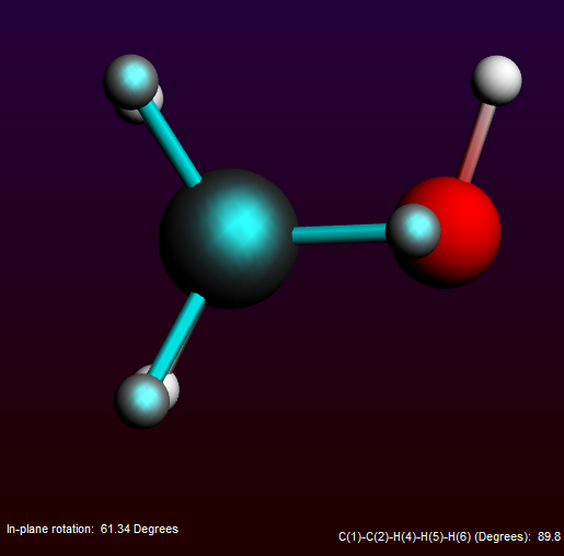
We are now trying to make an eclipsed geometry.

ctrl-Click with the left mouse button in one of the selected hydrogens,

and drag around to rotate the selection in-plane.

Rotate the hydrogen atoms in an almost eclipsed position.

You can move the selection by clicking in a selected object, and dragging with the mouse. All usual operations are possible: rotate, rotate in-plane, translate and zoom. Zoom in this case means moving the selection perpendicular to the screen.

In the status field you see the current rotation angle.

You have to click and start dragging at a selected item. If you click and drag in space you will move the entire molecule.

Getting and setting geometry parameters¶

Bond length¶

First select the oxygen atom and the connected hydrogen atom.

This time we make the selection by dragging a rectangle around all objects that we want to select.

Using the left mouse button together with the shift key, drag a rectangle

around the oxygen and hydrogen atom.

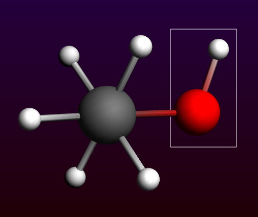
Release the mouse button (and the shift key)

The oxygen atom and the hydrogen atom are selected.

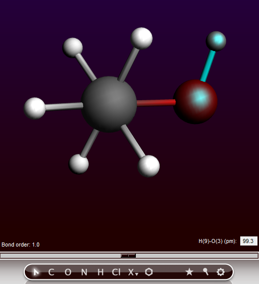
In the status area you see the distance between the selected atoms, information about the bond, and a slider.

You can set the distance to any value you wish by editing it, or (most conveniently) by using the slider.

Normally the smallest group of atoms will move to create the requested distance. If you press the control key while using the slider the last atom selected will be in the group of atoms to move.

Use the slider to move the H atom

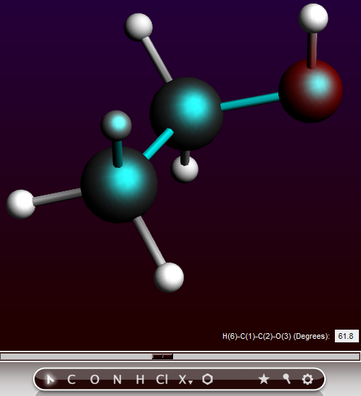
Bond angle¶

Select first one of the top hydrogens by clicking on it

Next, extend the selection (shift key) by clicking on the top carbon atom

Finally, extend the selection (shift key) by clicking on another top hydrogen atom

In the status area information about the bond angle of the selected three atoms is given, and the slider is again visible. You can change this value to a value you like, most conveniently using the slider.

Dihedral angle¶

By selecting four atoms we get information about the dihedral angle. And of course you can also change it, again most conveniently using the slider.

Move the molecule such that you can see all atoms

Select first one of the top hydrogens by clicking on it

Next, extend the selection (shift key) by clicking on the top carbon atom

Next, extend the selection (shift key) by clicking on the next carbon atom

Finally, extend the selection (shift key) by clicking on the oxygen atom

Coordinates¶

To view the coordinates we have to go to a different input panel. The input panels can be selected using the panel bar on the top of the input panels, the right half of the window.

In the right side of the ADFinput window:

Click on the Model tab in the panel bar

Select the Coordinates command

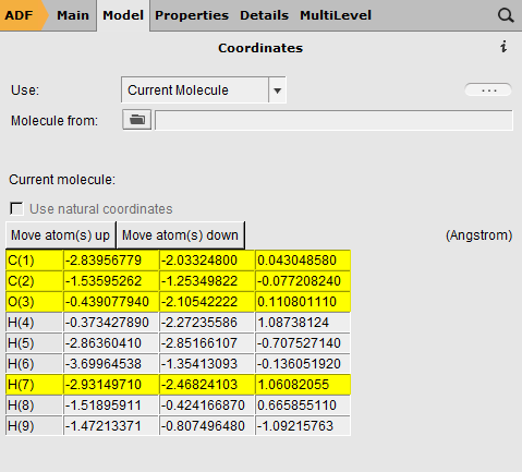
You get a list of all Cartesian coordinates. They will be updated in real time when you make changes to the molecule, and you can also edit the values yourself. In that case, the picture of the molecule will be updated automatically.

Note that some atoms are highlighted. These are the currently selected atoms.

The ‘Move Atom(s)’ buttons will move the selected atoms up or down. In this way you can re-order the atoms.

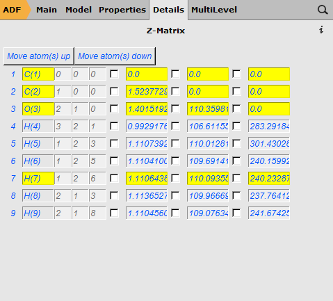
You may, in some cases, wish to use Internal coordinates. These will be updated in real time as well, and you can also edit the values yourself. If you re-order the atoms while using the Internal coordinates, the Z-matrix will be recalculated from scratch. The Z-matrix panel is in the Details tab, but we will use the search option to get to it:

Click the search icon at the right of the panel bar

Enter the text “z-ma” in the search field

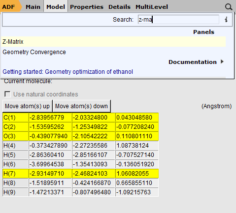
Note that in the search results the Z-Matrix panel is highlighted, and note that the search is not case sensitive.

Click on the selected option (Z-Matrix), or use the return key

Extending and changing your molecule¶

Before making some changes, let’s re-optimize. We first select the ‘Main’ panel so the coordinates will not be visible during the pre-optimization. Otherwise this may slow down the pre-optimization.

Click on the “Main” tab

Click on the pre-optimize button

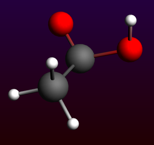
Let’s try to change the CH2OH group in a COOH group.

Thus, we need to:

• remove one hydrogen
• change one hydrogen into an oxygen
• change a single bond into a double bond

After this, we will revert to the ethanol molecule.

Delete an atom¶

First: delete one hydrogen

Click in empty space to clear the selection

Click once on the hydrogen to delete, it will be selected

Press the backspace key

The selected atom is removed.

Change the type of an atom¶

Next, we will change a hydrogen into an oxygen atom

Select the O-tool (or press the ‘O’ key)

Double-click on the hydrogen that should change into an oxygen

Change the bond type of an existing bond¶

Now the oxygen atom is singly bonded to the carbon, we need to change this into a double bond.

Click on the bond between the carbon and the new oxygen

Use the Bonds → Bond Order → Double menu command (or just press the ‘2’ key)

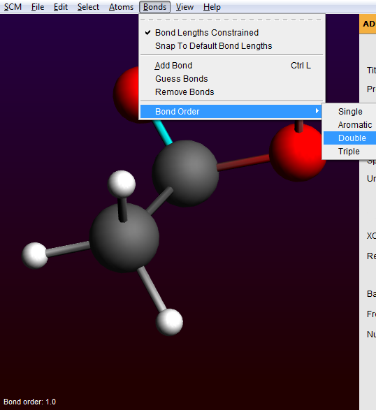
The single bond has changed into a double bond.

Another way to modify a bond type is to click on the bond once which will select this bond. Then click on the bond tool in the menu bar (‘ball and stick’ logo to the right of the start), and select the proper bond type.

The fastest way to change the bond order is to use the keyboard shortcuts. If you have selected a bond, press 1 for a single bond, 2 for a double bond, 3 for a triple bond and 4 for an aromatic bond.

To get a reasonable geometry optimize the structure:

Click in empty space to deselect the bond

Press the pre-optimize button

If not converged, press pre-optimize again

Add new (bonded) atoms¶

Now, to revert to the ethanol molecule, we first remove the new doubly-bonded oxygen atom, and then add one hydrogen atom.

Click once on the doubly-bonded oxygen atom to select it

Press the backspace key to delete it

Select the H-tool (or press the ‘H’ key)

Click once on the carbon atom connected to the oxygen

Note that this way you started bonding mode again, as indicated by the bond to the mouse position.

Click once in empty space to make a hydrogen atom (connected to the carbon!)

Click once on the just created atom to stop bonding

Repeat this to add a second hydrogen to the carbon atom

Pre-optimize the molecule

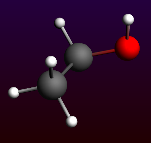
Once again you have created an ethanol molecule.

Preset¶

You should always start by choosing the proper preset.

ADF has many different modes of operation. ADFinput presents the correct settings for some common calculations together as ‘presets’.

So to optimize the geometry of the ethanol molecule we choose the proper preset:

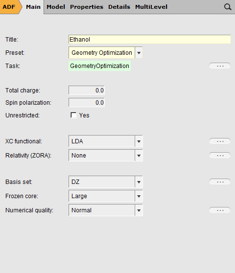
Select the ‘Geometry Optimization’ preset from the ‘Preset’ menu.

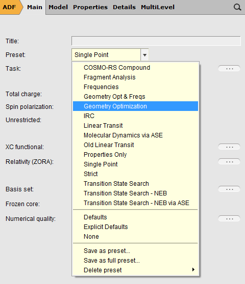
Presets might change any number of input options. In this particular example, the main Task will change from ‘Single Point’ to ‘Geometry Optimization’. You can easily see what fields have been updated by a preset: they are colored green.

If you would use this preset again later, the input values that are set by this preset will revert to the default values. If you made changes to those fields you will lose those changes.

Title¶

This field, currently empty, has no special meaning for the calculation routine. It will be used as an identifier for your convenience in the result files of the ADF calculation. In this case, let’s set the title to the name of the molecule:

Enter ‘Ethanol’ without quotes in the ‘Title’ field.

Note that as soon as you start typing in the title field, the color of the field changes to yellow. The yellow color here and in other cases indicates that you have made a change with respect to the default value for this field.

XC functional¶

An important input option is the XC functional to use.

For this tutorial the default potential during the SCF is sufficient. So just leave this at the default value. For more accurate results you should select a better XC potential.

Basis set¶

With the ‘Basis Set’ pull-down menu you select the basis set you want to use.

The menu gives access to the basis sets regularly used.

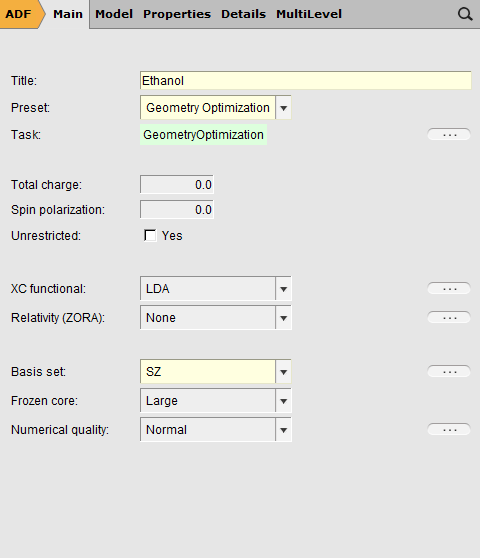
For this tutorial we will choose a very small basis set. This will yield less accurate results, but the calculation runs much faster. Obviously, if you want more accurate results you should use a better quality basis set. Thus:

Select ‘SZ’ from the ‘Basis Set’ pull-down menu

Numerical quality¶

The ADF software package uses a numerical integration scheme for virtually everything it may calculate. A numerical integration scheme generates some kind of grid (and corresponding weights). ADF and BAND have always been using the teVelde (Voronoi) integration scheme. For many calculations the Becke integration grid works better, so in ADF2013 the Becke integration grid method has been added. It now is the default method, and normally you should use the Becke grid option.

Another numerical detail is that a density fit is used, for computational efficiency. The spline Zlm fit is now the default fit method, the old slater type fit is still available.

With the Numerical quality option you can select the quality of both the Becke integration and the spline Zlm fit at the same time.

Increasing the quality makes the results more accurate, but will require substantially more computation time.

Similarly, decreasing the quality will result in less accurate results, but you may get results faster.

The default value will in most cases be fine, certainly for this tutorial. If you go to the Details section (click on the ...) you can set details of the integration scheme and fit method. However, the Numerical quality option in the main panel is the most convenient way to select the quality.

Other input options¶

The panels on the right side contain many more input options. You select a panel with the menus in the panel bar, or by searching for a particular option (as we did to locate the Z-Matrix panel). When searching for an option, any text in the panels will match, as well as from the help balloons. Also the corresponding ADF input keys will match.

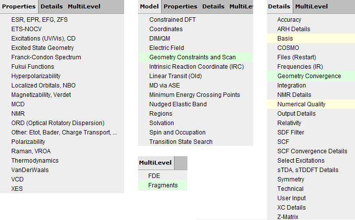
The menu items use a color coding to show you which panels have been affected by a preset (green), by the user (yellow), or both (red).

As we will not do anything special right now, you do not need to change anything in other panels.

Save your input and create a job script¶

Finally you will want to save your input.

Select the File → Save command.

Enter the name ‘ethanol’ in the Filename field.

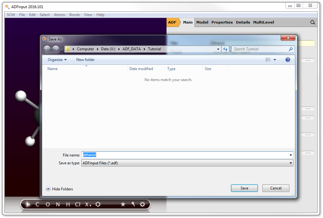
Click on Save

Now you have saved your current options and molecule information. The file will automatically get the extension ‘.adf’.

ADFinput has also created a corresponding script file. This script file has the same name, but with an extension ‘.run’ instead of ‘.adf’.

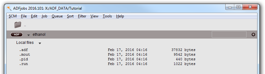
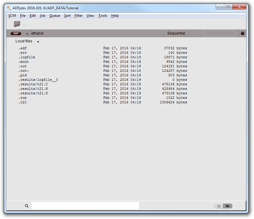
In the ADFjobs module you can see what files have been created:

Click once in the ADFjobs window to activate it

Click once on the triangle in front of the name of the job (ethanol)

You will see the .adf and .run files, and a .pid file that ADFjobs uses to store information. You might also see the picture that you saved, if you used the name ‘ethanol’ for it. Only the extensions are listed, so the real filenames are ethanol.adf, ethanol.run and ethanol.pid. Notice the job status icon (the open circle on the right) that ADFjobs uses to indicate a new job.

Run your calculation¶

To actually perform the calculation (the geometry optimization of the ethanol molecule), use the Job → Run menu command in ADFjobs:

Make sure the ethanol job is selected in ADFjobs (it is if you followed the tutorial)

Select the Job → Run command

This will execute the run script that has just been created. If you have never made changes in the ADFjobs setup, the default behavior is to run the job in the background on your local computer, using the Sequential queue. This queue will make sure that if you try to run more then one job at the same time, they will be run one after another.

Once your job starts running, ADFjobs will show the progress of the calculation: the last few lines of the logfile:

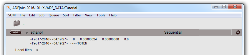
Note that while running, the job status symbol in ADFjobs changes.

If you wish to see the full logfile while the calculation is running, just click on the logfile lines displayed in the ADFjobs window:

Click on the logfile lines in the ADFjobs window

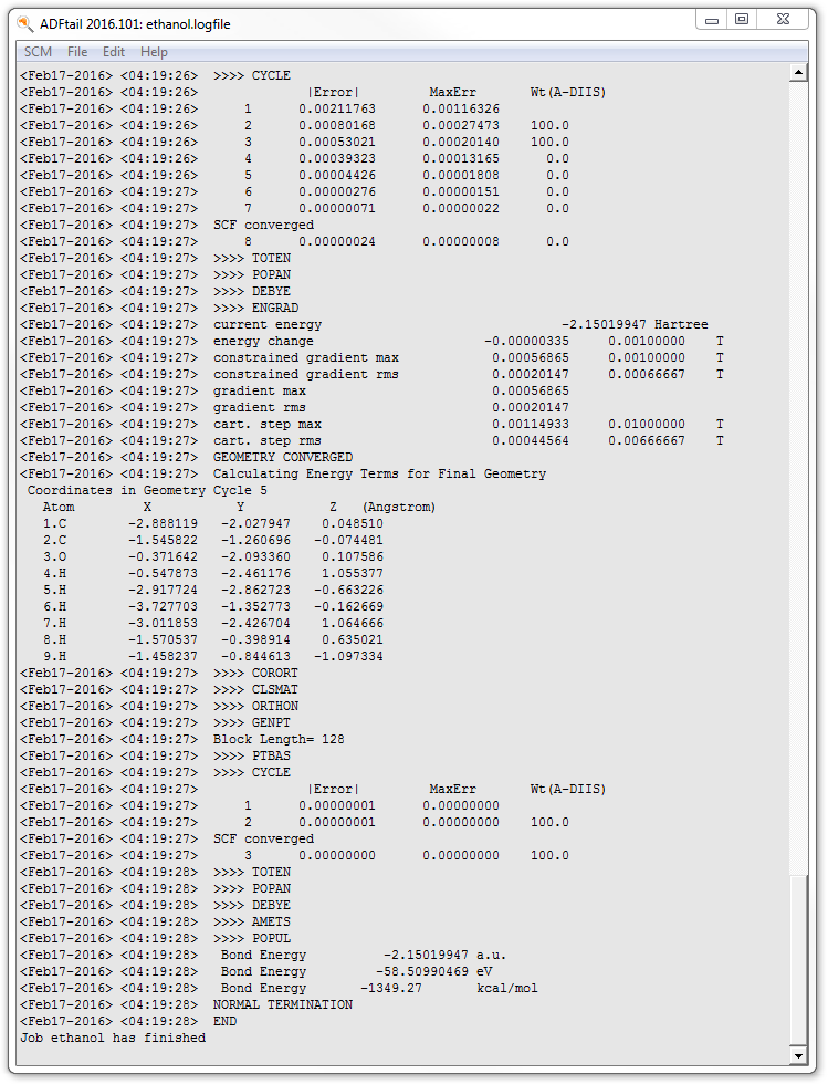
Now the logfile is showing in the ADFtail window:

Logfile: ADFtail¶

The logfile is saved and extended by ADF as it is running. Normally it is most convenient to view it only in the ADFjobs window to prevent screen clutter.

Right now it is already showing in the ADFtail window, and in the ADFjobs window, but you could have used any text editor.

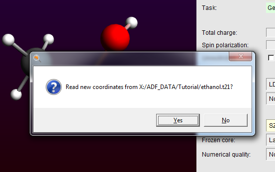
Wait for the calculation to finish:

Wait until ADFtail shows ‘Job ... has finished’ as last line

In the dialog that pops up, click ‘Yes’ to update the geometry

Now close ADFtail by using the File → Close menu command:

In the window showing the logfile (the ADFtail window):

Select the File → Close command

In the ADFjobs window, note that the job status icon has changed to indicate that the job is ready:

Files¶

ADF has created a couple of data files and a couple of text files. You can check this in the ADFjobs window:

Click on the ADFjobs window

Note that the Local files are visible because earlier in the tutorial you already clicked on the triangle opening the details for this job.

The .adf file is the input as saved by ADFinput.

The .run file is the run script, also saved by ADFinput.

To enable specific options of your ADF job, changes to the text of the .run script can be made opening it via double-click. A separate text editor window pops up after the double-click (the non-default text editor program can be defined via the $EDITOR variable passed to ADF-GUI). When you run your job, your edited .run file will be used. Note that when you save your input via ADFinput again, your .run file will be overwritten (and thus you lose any changes you made when editing the .run file).

The .job file is a script file based on the .run file, and is created by ADFjobs. It contains all commands required to run your job, and is actually run by ADFjobs when you use the Run command.

The .pid file is a file that contains your job status and configuration. It is used by ADFjobs.

The other files are produced by ADF. The .err file contains error messages, the .logfile shows the progress of the calculation, the .out file is the main (text) output file, and the other files are binary files that store results of the calculation.

Geometry changes: ADFmovie¶

ADF has optimized the geometry, and we can use the ADFmovie module to visualize the progress of the optimization. So let’s start ADFmovie using the SCM menu in your ADFinput window:

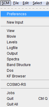
Select the SCM → Movie command in ADFinput

The ADFmovie module will display a movie of the geometry optimization.

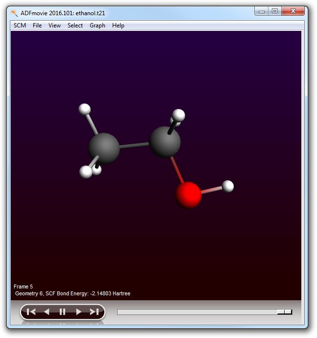
To step through the different geometries, use the slider below the picture. Clicking in the slider will single step through the frames. Alternatively you can grab the slider and move to the frame you wish, or you can use the left and right arrow keys to single step through the frames.

You control playing with the buttons. When your mouse pointer is above any of the buttons, and not moving, a balloon will pop up showing what that particular button will do.

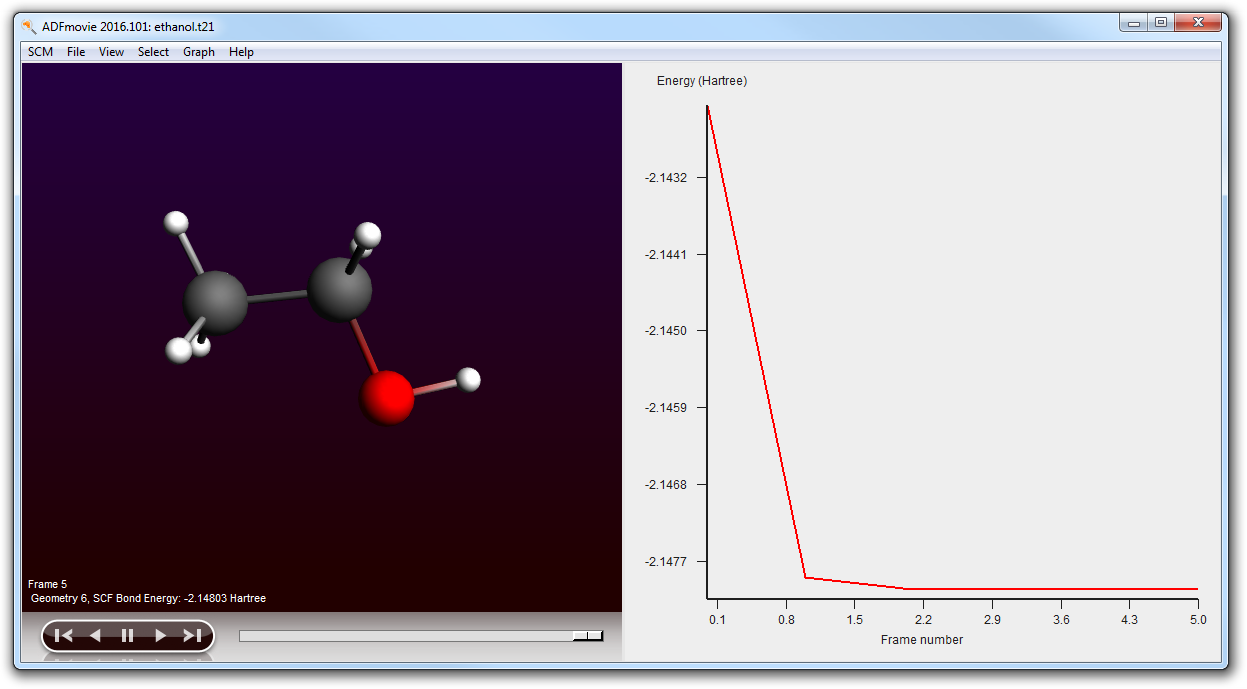
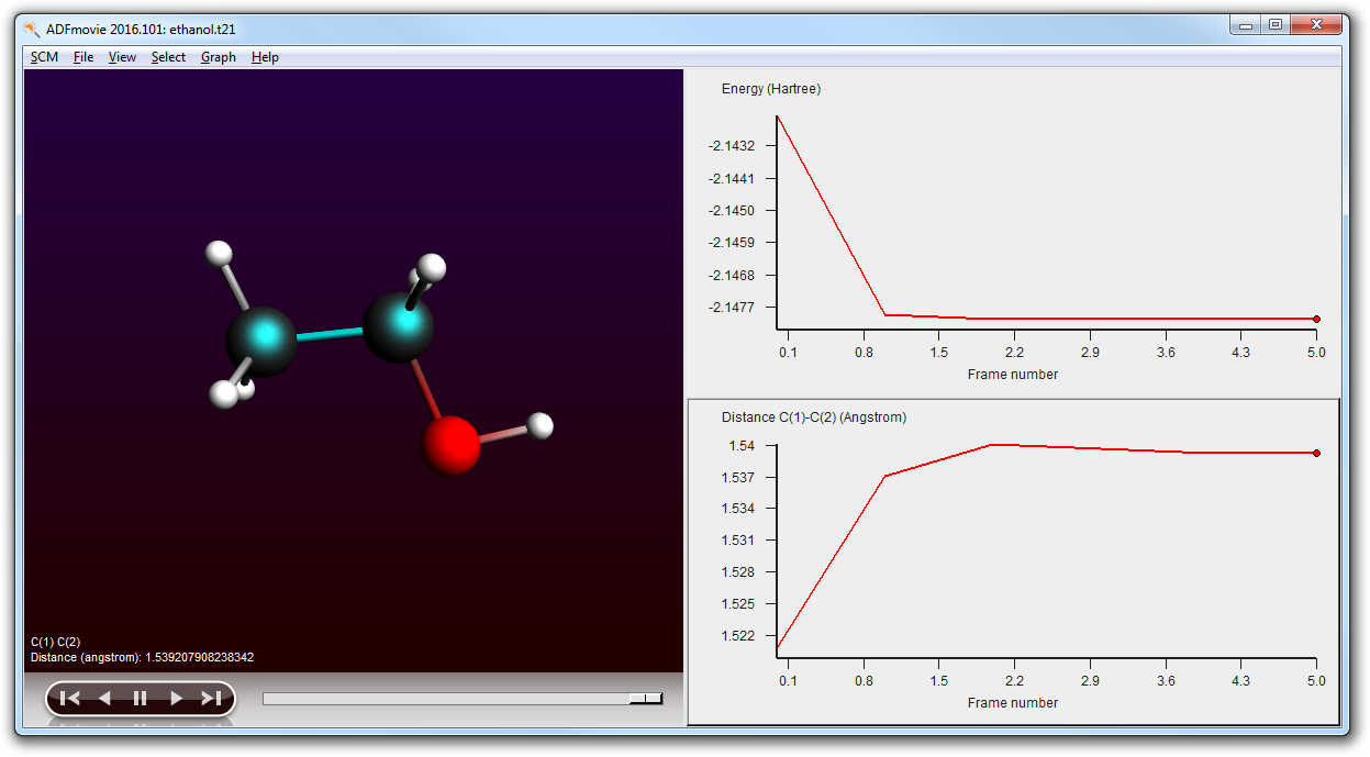
It is often nice to have a graph of the energy as function of the geometry step. ADFmovie can show such graphs easily:

Use the Graph → Energy menu command

You can even show several graphs for different properties at the same time:

Use the Graph → Add Graph menu command

Select two carbon atoms by shift-clicking on them

Use the Graph → Distance, Angle, Dihedral menu command

Now you have two graphs. One of them is the ‘active’ graph. When you make a new graph it will always be the active graph. You can also make a graph active by clicking on it.

When you select a property from the Graph menu (Energy, Distance and so on) that property will be plotted in the active graph.

You can also have multiple curves in one graph, if possible: one property per Y-axis. You may have several curves on the same Y axes if they are using the same unit (all Angstroms for example):

Select two carbon atoms and one oxygen atom by shift-clicking on them

Use the Graph → Distance, Angle, Dihedral menu command

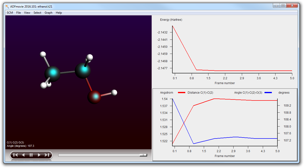
Another feature is that you can click on a point in one of the graphs. It will be marked, the movie will jump to that particular step, and if you have more then one graph the corresponding point(s) will also be marked in the other graphs.

To rotate, translate, or zoom the picture, use your mouse, just as in ADFinput.

Use the slider to go to a frame in the middle of the optimization

Selecting atoms provides information about atoms, bonds, etc. The information will be updated when you go to another point in the movie (a different geometry). You can see examples of these in the pictures above.

You can also show this information in the 3D window:

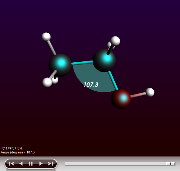
Use the View → Geometric Info → Angle menu command

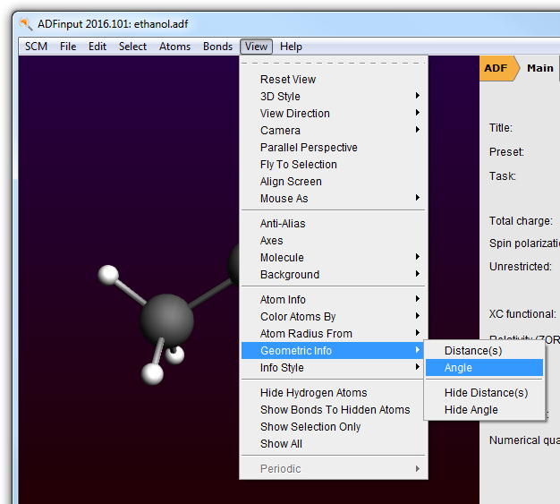
The angle will be visually added to your molecule :

In the ADFmovie window: select File → Close

Orbital energy levels: ADFlevels¶

Select your job in the ADFjobs window by clicking on the job name

Select the SCM → Levels command

ADFlevels will start and show a diagram of the energy levels of the ethanol molecule.

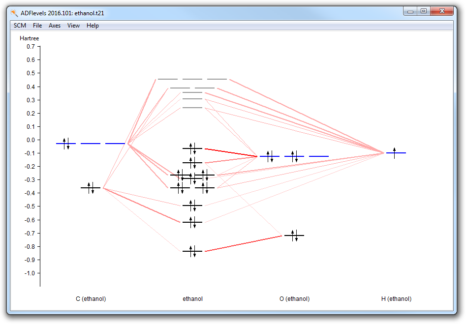
In the diagram you can see from what fragment types the molecular levels are composed.

Move the mouse around, above different levels, without clicking

Balloons will pop up with information about the level at the mouse position: The MO number, eigenvalue, occupation, and how it is composed of SFOs (fragment orbitals).

Click and hold on the HOMO level of the molecule

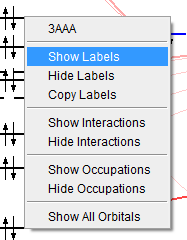
In the pop-up that appears, select ‘Show Labels’

Click and hold on the HOMO of the O fragment type

In the pop-up, select ‘Show Labels’

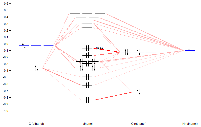
To actually see the orbital, select the orbital from the top of the pop-up menu:

Click and hold on the HOMO level of ethanol

Select the ‘3AAA’ command

A window with a picture of the orbital should appear.

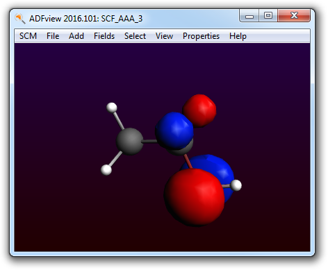
You can move (rotate, translate and zoom) the orbital with your mouse.

Close the window showing the orbital: File → Close (in the window displaying the orbital)

Electron density, potential and orbitals: ADFview¶

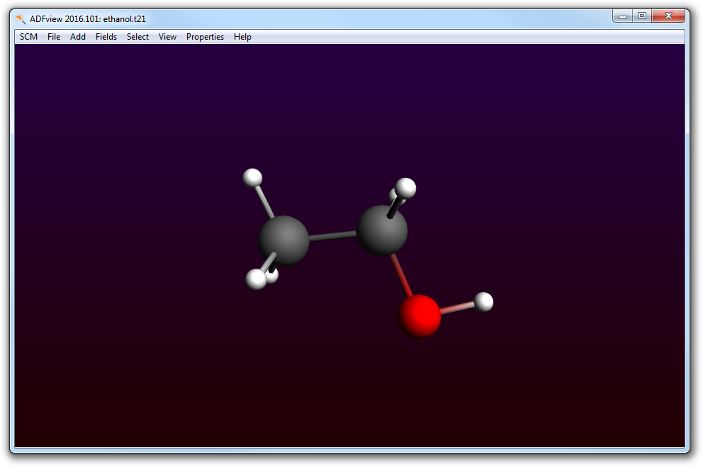
Select SCM → View

ADFview will start up and show a picture of your molecule:

You can use ADFview to visualize all kinds of ‘field’ related properties: densities, orbitals, potentials, etc. You actually have already used it before: the picture of the orbital that was created using ADFlevels was shown by ADFview.

Use the mouse to rotate, translate or zoom, as in ADFinput.

In the Properties menu there are some pre-defined things to visualize: density, spin-density, HOMO, LUMO and more. If you select one of these, you will see the corresponding item immediately. However, ADFview can do much more and gives you lots of control.

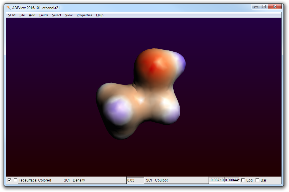
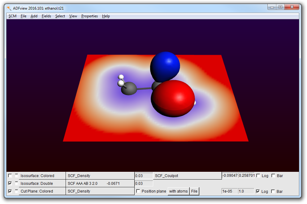
For example, lets show a density isosurface, colored by the electrostatic potential:

Select the Add → Isosurface: Colored command

Below the picture a control line will be created. ADFview creates one such line for all visual items and special fields (surfaces, cut planes, calculated fields, etc.) that you add.

In this particular case the control line contains two pull-down menus that you use to select the fields that you want to visualize.

From the first pull-down menu in the control line, select Density → SCF

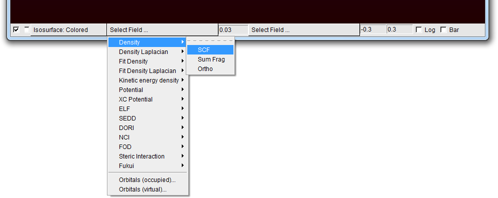
From the second pull-down menu in the control line, select Potential → SCF

To demonstrate some other possibilities of ADFview, do the following:

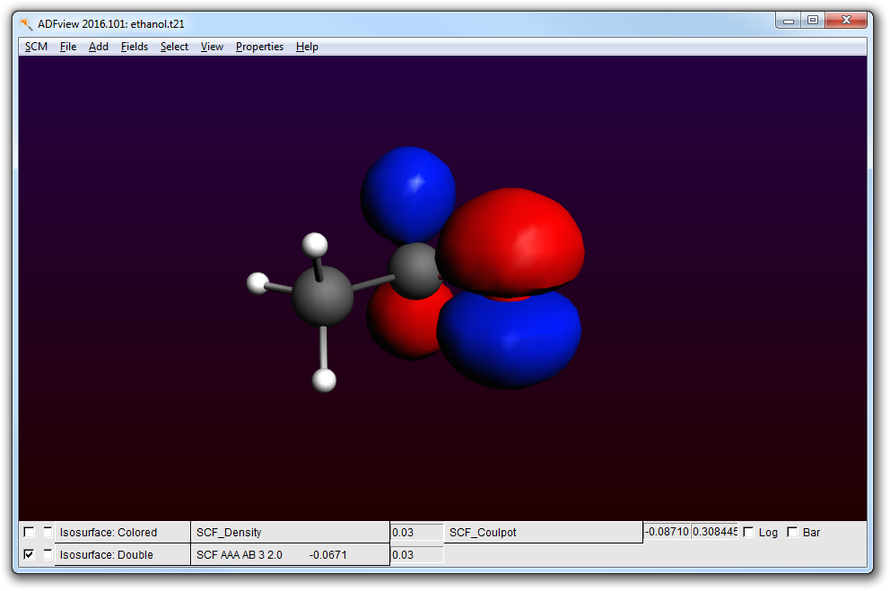
Select the Properties → HOMO command

Click on the check box in the FIRST control line to hide the density

Rotate the molecule to get a good view

Select the Add → Cut plane: Colored command

In the new control line, press on the pull-down menu and select Density → SCF

Click the check box in front of the ‘Isosurface: Double’ line to hide the HOMO

Select the Carbon and Oxygen atoms (three atoms)

Click the ‘with atoms’ button next to the ‘Position plane’ option (thus the button, not the check box)

Click the check box in front of the ‘Isosurface: Double’ line to show the HOMO

Select the Fields → Grid → Medium command

Click Yes to recalculate the fields

Rotate your molecule to get a good view

You can save the picture you create using the Save Picture menu command:

Select File → Save Picture ...

Enter the name (without extension) of the file you want to create

Click Save

A picture with the (file)name you specified has been created.

You might want to explore some more of the possibilities of ADFview on your own. Many different properties can be visualized as you probably have noticed in the pull-down menus. Be careful with activating Anti-Alias: it makes the pictures even better, but also slows ADFview down significantly.

Browsing the Output: ADFoutput¶

The output file (tutorial.out) is a plain text file. You can view it with your favorite text editor (or text viewer). You can also use the ADFoutput GUI module which provides a convenient way to check the results:

Select the SCM → Output command

Select the Iterations → Geometry Cycles command

The ADFoutput program will start showing the results of your calculation, and via the menu you jumped to the first section with geometry details:

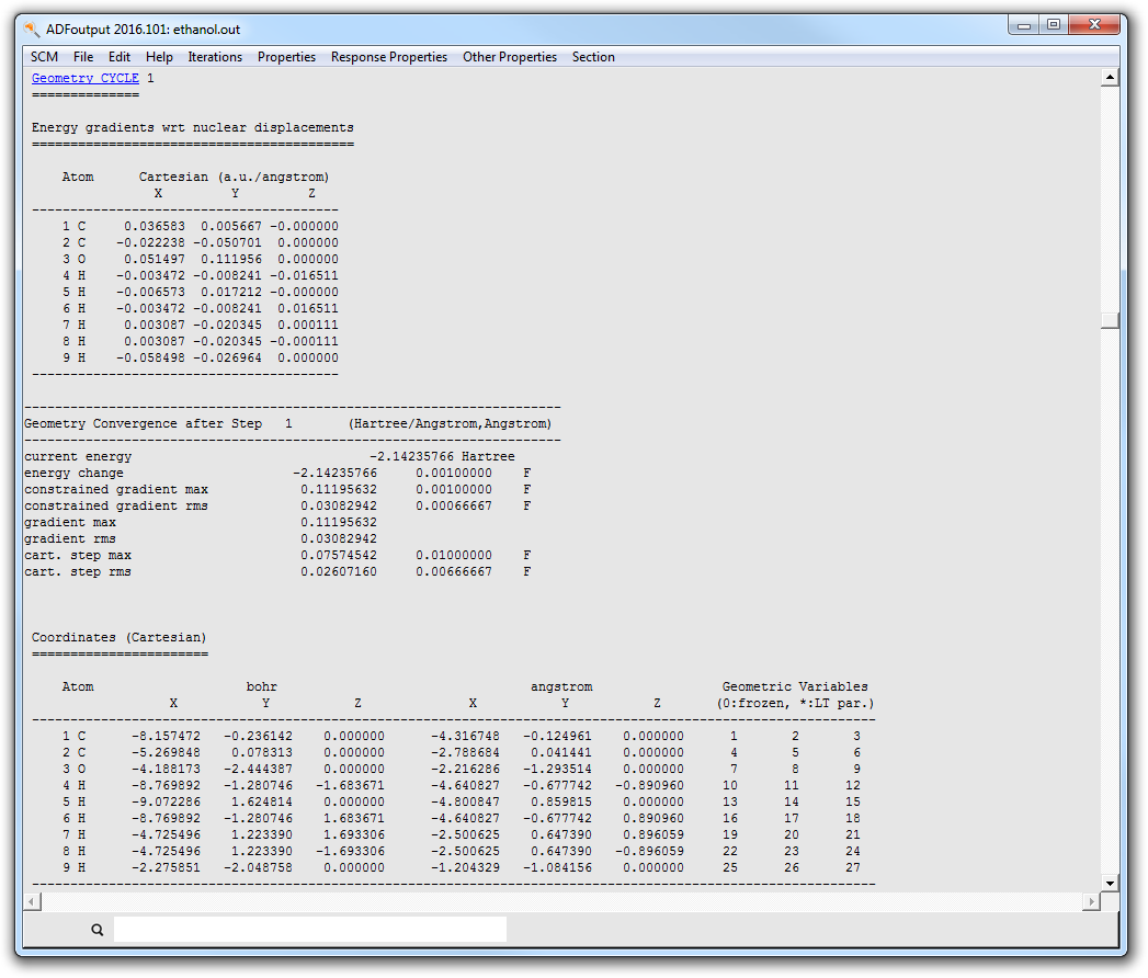
You can use the menus to go to different parts of the output file, or you can just use the scroll bar. If a menu option is shaded, this means that no corresponding section of the output is available.

Clicking an output section title highlighted in blue will skip to the next section with the same title, if present.

As we are now done with tutorial 1, close all windows that belong to this tutorial:

Select the SCM → Quit All command in any ADF-GUI window

All open windows from the ADF-GUI will be closed.