Bandstructure/DOS/Charges/Orbitals/Densities - With a Grain of Salt¶

Step 1: Start ADFinput¶

Start ADFjobs

We prefer to run the tutorial in a new, clean, directory. That way we will not interfere with other projects. ADFjobs not only manages your jobs, but also has some file management options. In this case we use ADFjobs to make the new directory:

Select the File → New Directory command (thus, the New Directory command from the File menu)

Rename the new directory by typing ‘BandTutorial’ and a Return

Change into that directory by clicking once on the folder icon in front of it

Now we can start BANDinput using the SCM menu:

Use the SCM → New Input menu command

Switch to BAND mode (panel bar ADF → BAND)

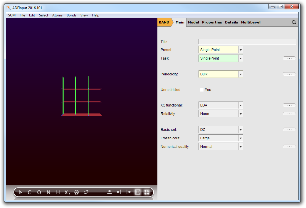
The BANDinput window consists of the following main parts:

• the menu bar with the menu commands (File, Edit, ...)
• the drawing area of the molecule editor (the dark area on the middle left side)
• the status field (lower part of the dark area, blank when the ADFinput is empty as shown above)
• the molecule editor tools
• many panels with several kinds of options (currently the ‘BAND Main’ panel is visible)
• panel bar with menu commands to activate the panel of choice
• a search tool (at the right of the panel bar)

In the drawing area you see the lattice vectors, with three repetitions of the unit cell along each vector. The first lattice vector is red, the second green, and the third blue. Using the View Periodic menu you can change the display of the periodic images:

View → Periodic → Repeat Unit Cells

If you look in the toolbar with molecular editor tools, you see that the rightmost button is no longer glowing. You can also use this button to toggle the display of the periodic images:

Click once on the rightmost button in the toolbar (the four dots)

Now you should see the periodic repetitions again.

Step 2: Set up the unit cell¶

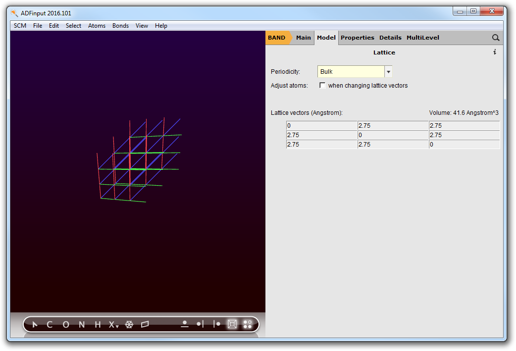
Salt has an fcc lattice. First we need to set the lattice vectors:

Panel bar Model → Lattice

Enter the lattice vectors, as shown below

Step 3: Add the atoms¶

Now we will add the Na and Cl atoms. It is convenient to turn of the periodic display while doing this:

Uncheck View → Periodic → Repeat Unit Cells

Click on the X tool, and select Na

After this you see at the bottom of the screen “Na tool” in the status field:

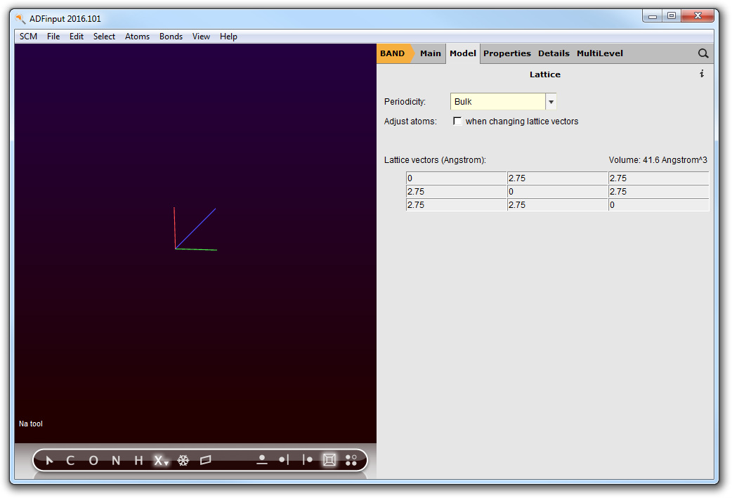
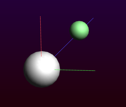
Click once in the drawing area, near the origin

Click once on the created atom to stop bonding

As you can see the atom is not exactly in the origin. This can be fixed if you wish:

Edit → Set Origin

To add the Cl atom you can proceed the same way:

Select the Cl tool (via the X button again)

Click once somewhere in the unit cell

Click on the new Cl atom to stop bonding

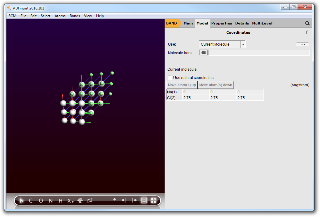
Next you should edit the Cl coordinates and change the Cl color:

Select the coordinates panel: panel bar Model → Coordinates

Change the Cl coordinates to be (2.75,2.75,2.75)

Check View → Periodic → Repeat Unit Cells

Now your system looks like:

Step 4: Running the calculation¶

If you wish so, you can give your calculation a title:

Panel bar Main

Enter NaCl in the “Title” field

File → Save, name it “NaCl” and press Save.

File → Run

The progress of the BAND calculation is visible in the ADFjobs window (a few lines of the ‘logfile’). (the ‘logfile’). After a few minutes the calculation has finished, and it looks like:

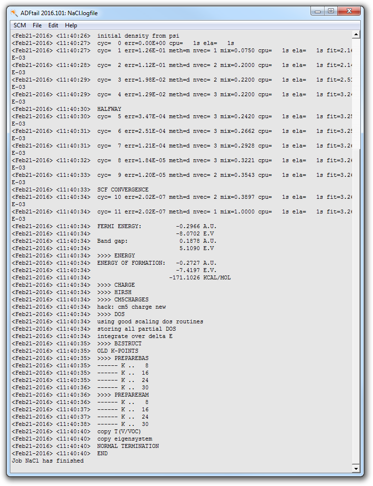
Wait for the text ‘Job NaCl has finished’

The calculation has produced two important result files: “NaCl.out”, which contains the result of the calculation in text format, the second is”NaCl.runkf” which is a binary result file.

Step 5: Examine the band structure¶

SCM → BAND Structure

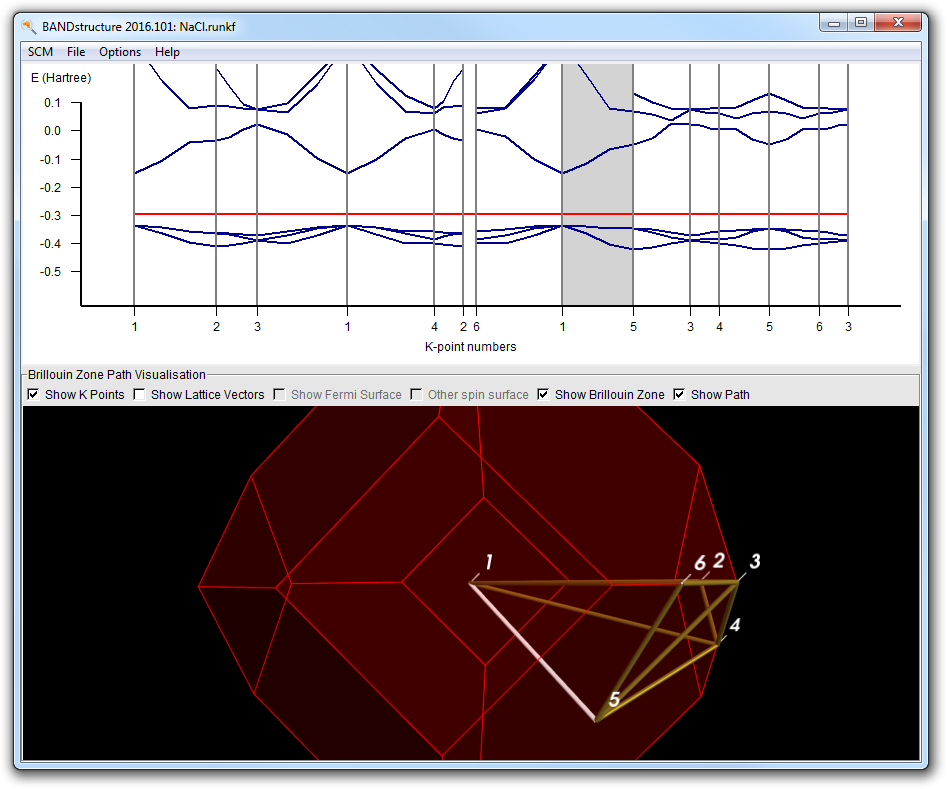
This will open the bandstructure window:

It consists of a plot and a picture of the Brillouin zone. In the plot the red line is the Fermi level. Below the Fermi level are four occupied bands. You can see this more clearly by vertical zooming:

Click on the right mouse button, and drag the pointer up to zoom vertically

When the region of interest gets out of view, drag it into view (with the left mouse button)

The bottom part of the plot will look like:

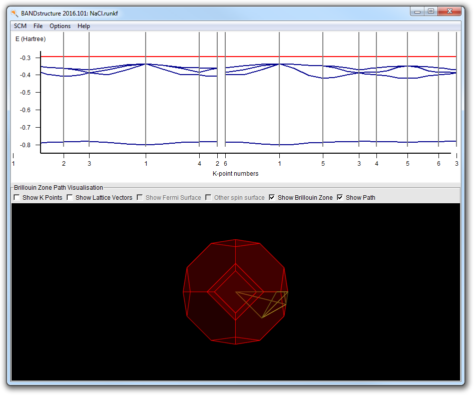
In most k-points you see now four bands below the Fermi level. In some k-points you see fewer because they are degenerate.

Now you may wonder about the path taken through the Brillouin zone. This is where the bottom part comes in handy. You can zoom and rotate, just as with molecules in BANDinput.

Zoom in a bit, by using the scroll wheel on your mouse or pressing the Middle button and moving upwards

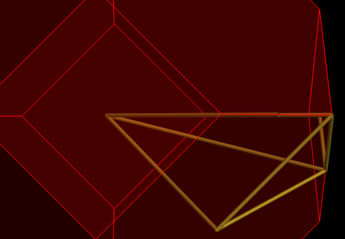
Toggle the button to display the k-points

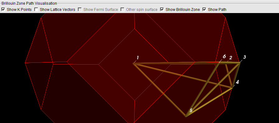
Now click on the line from 5 to 1

Note how the line lights up, and also how the corresponding segment is indicated in the plot by a gray background. You can also click on the plot to select line segments.

Rotate the Brillouin zone a bit to convince yourself that the line (from k-point 5 to 1) runs from the center to the center of a hexagonal face.

Step 6: Visualizing the results¶

Plotting the orbitals¶

Now what is the character of the bands? Let us first examine this narrow band at about -0.5 Hartree.

SCM → View

In ADFview: Add → Isosurface Double (+/-)

In the bar at the bottom of the window, you can select which field to show.

Select Occupied Orbitals in the Select Field pull-down menu

Select the lowest band (k=0,0,0) (the topmost in the Occupied Orbitals window)

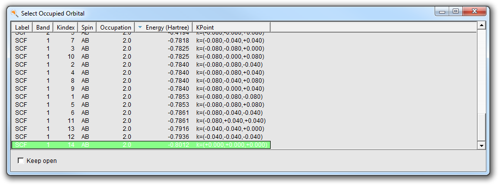
From the label you can see that it has an energy of -0.8012 and the coordinates are (0,0,0).

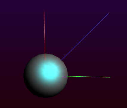
A progress bar will appear, and after a while you will see the orbital:

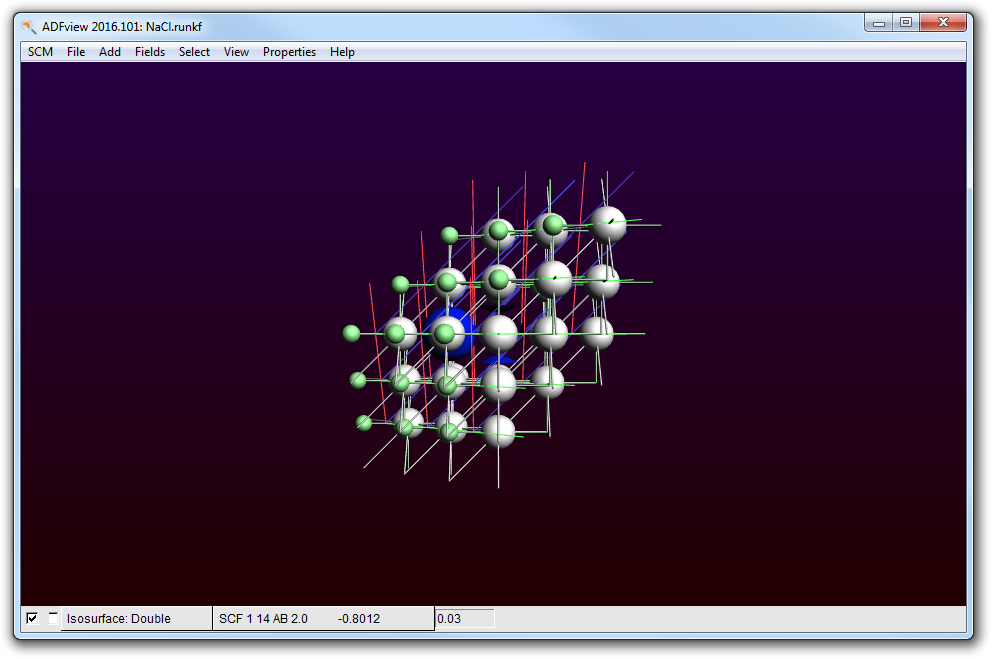
If you rotate it a bit and toggle the isosurface on and off (with the check box in front of it), you can convince yourself that this orbital is located around the small atom, which is the Chlorine.

Toggle the periodic view (the menu View → Periodic → Repeat Unit Cells)

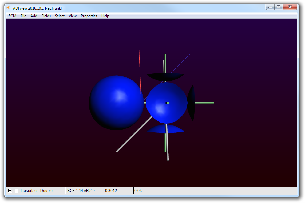
Obviously this is the 3s band of Cl. The strange truncated spheres are due to contributions of neighboring cells.

It is generally easier to interpret orbitals at k=(0,0,0), the gamma point. At the end of the list of occupied orbitals you find the other three orbitals in the gamma point. You can also sort the table by K point:

Click on the Kpoint header to sort by K point

Select the last occupied orbitals at k=(0,0,0), with the highest energy

Actually, the last three orbitals in the Gamma point are degenerate. Take a look at all three of them.

From these orbital pictures we can conclude that the valence band is indeed mainly of Chlorine-p character.

You may want to check the lowest orbitals of the (unoccupied) conduction band.

Plotting the partial density-of-states¶

There is in fact a much more easy way to conclude that the valence band is mainly of Chlorine-p character.

Open the DOS module: SCM → Dos

and a window like this will appear:

The Fermi energy is around -0.43, and there is clearly a gap. Just below it there is a valence band, and at -0.2 Hartree starts the conduction band.

Select the View → Add Graph command

(Now you see two plots of the total DOS)

Select with the mouse the Chlorine atom (the small green one)

It is already immediately clear that the valence band comes from the Chlorine, and the conduction band from the Sodium.

Right-click with the mouse on the selected Cl atom and

check the ‘P-DOS’ check box in the pop up menu.

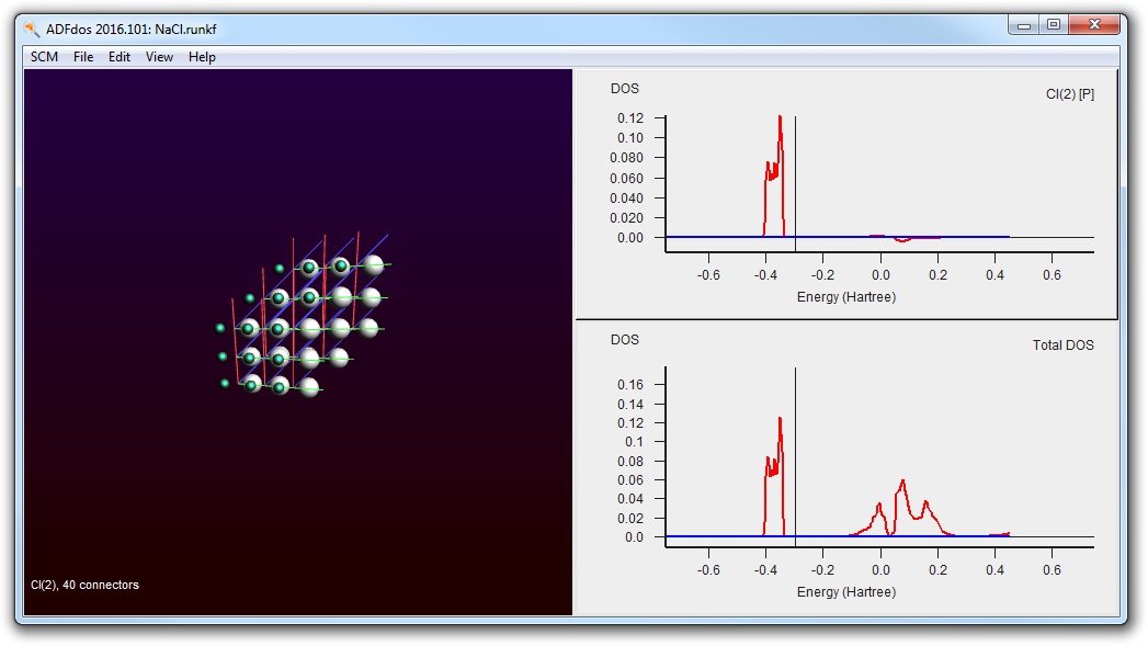
This shows that the valence band is clearly made of Chlorine p-orbitals.

Plotting the deformation density¶

Intuitively you might expect that the charge of Na should be +1 and from the Cl -1. This can be best seen by making a cut plane:

Go to ADFview (SCM → View)

Delete the double isosurface with the ‘Isosurface: Double’

pull-down menu in the bar on the bottom and select ‘Delete’

Add → Cut Plane: Contours (+/-)

Fields → Grid → Fine

Select the deformation density in the fields menu (in the Fit density sub-menu)

Check Log

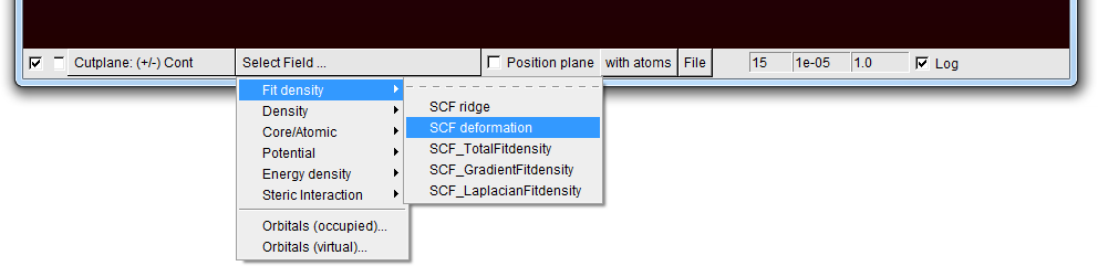
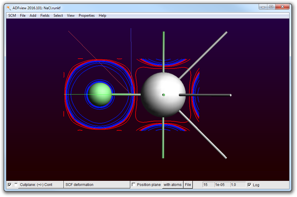
Indeed we see that charge is added (blue) near the Cl and removed (red) from the Na atom. The trend is good, but what is the total amount of charge transferred?

Step 7: Check the charges¶

Use the “Properties → Atom Info → Hirshfeld Charges → Show” menu command

This will show you

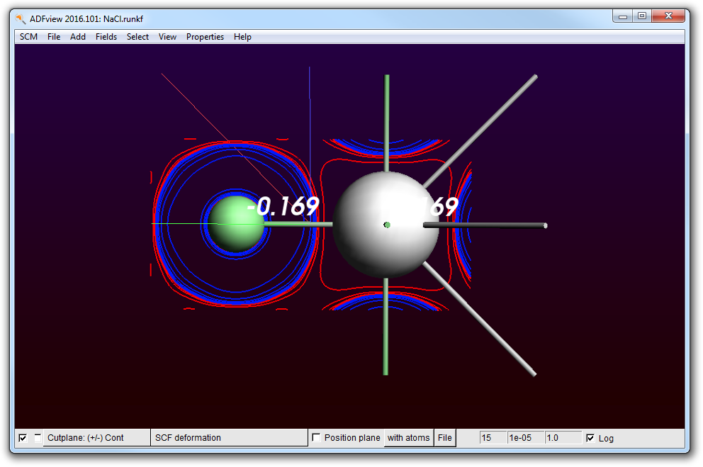
So the amount of charge transferred is only about 0.2. This is of course due to the fact that the Cl p-band overlaps quite significantly with the Na region.

The conclusion of this tutorial: we should take the idea that one electron is transferred from Na to Cl with a grain of salt.