
External Potentials with QET
Apply a prescribed MLPot.Vext profile across an fcc copper slab and inspect the z-resolved QET charge response.
Overview
QET is a charge-aware machine learning potential which uses a linear-scaling, analytically solvable charge-equilibration scheme.
In AMS, the per-atom MLPot.Vext atomic attribute can be used to apply an external potential profile to a chemical system by shifting the atom electronegativity used during charge equilibration. Its value is given in eV, matching the energy scale of the electronegativity term.
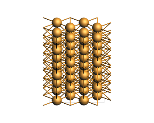
This example uses a small fcc copper slab. We prescribe a linear MLPot.Vext profile across the slab, from -1 eV on the bottom z-plane to +1 eV on the top z-plane, run a QET single-point calculation, and inspect the resulting atomic charges as a function of height. This is not intended as a production electrochemical setup; it is a compact demonstration of how an atom-wise external potential profile enters the QET workflow.
The important distinction is that MLPot.Vext is a prescribed atom-attached energy shift. QET responds to the profile you provide, but this example does not solve for a self-consistent electrostatic field or electrode boundary condition.
Imports
from collections import defaultdict

import matplotlib.pyplot as plt
import numpy as np

import scm.plams as plams
from scm.base import ChemicalSystem, Lattice
from scm.inputs import AMS, MLPotential
from scm.plams import AMSJob, Settings, finish, init, view
Build a copper slab
The slab is periodic in the two in-plane directions and uses an fcc conventional-cell basis. We group atoms by their unique z-coordinate and assign a linear MLPot.Vext profile from the bottom z-plane to the top z-plane. This keeps the example close to a normal copper slab while making the applied potential profile explicit in the atom attributes.
slab = ChemicalSystem()
lattice_constant = 3.61
nx, ny, nz = 2, 2, 3
basis = [
    (0.0, 0.0, 0.0),
    (0.0, 0.5, 0.5),
    (0.5, 0.0, 0.5),
    (0.5, 0.5, 0.0),
]

for ix in range(nx):
    for iy in range(ny):
        for iz in range(nz):
            for bx, by, bz in basis:
                slab.add_atom(
                    "Cu",
                    coords=(
                        lattice_constant * (ix + bx),
                        lattice_constant * (iy + by),
                        lattice_constant * (iz + bz),
                    ),
                )

slab.lattice = Lattice(
    [
        (lattice_constant * nx, 0.0, 0.0),
        (0.0, lattice_constant * ny, 0.0),
    ]
)
slab.enable_atom_attributes("mlpot")

z_planes = np.array(sorted({round(atom.coords[2], 8) for atom in slab.atoms}))
vext_by_z = dict(zip(z_planes, np.linspace(1.0, -1.0, len(z_planes))))
for atom in slab.atoms:
    atom.mlpot.Vext = vext_by_z[round(atom.coords[2], 8)]

view(slab, width=500, height=420, fixed_atom_size=False, config=plams.ViewConfig(normal=(0, 1, -0.4)), guess_bonds=True)
QET settings
The QET model is provided by the MatGL backend. We explicitly request atomic charges so that the charge response to the prescribed MLPot.Vext profile can be read from the results.
settings = Settings()
settings.input = AMS(Task="SinglePoint")
settings.input.Properties.Charges = True
settings.input.Engine = MLPotential(Backend="MatGL", Model="QET-PBE-2025")
settings.runscript.nproc = 1
Run the slab calculation
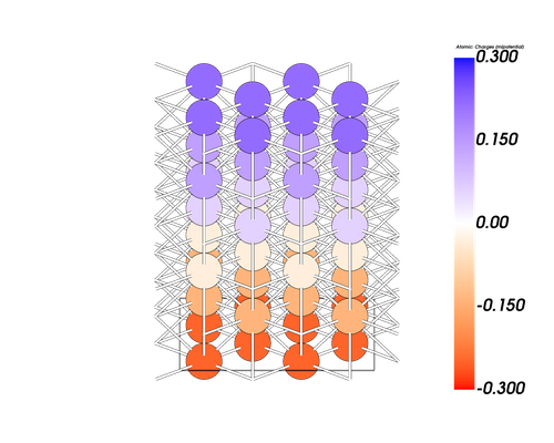
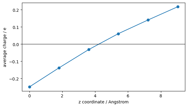
The total charge remains zero. The prescribed external potential profile increases monotonically from the bottom z-plane to the top z-plane, so QET redistributes charge while preserving overall charge neutrality.
job = AMSJob(molecule=slab, settings=settings)
results = job.run()
if not results.ok():
    raise RuntimeError(results.get_errormsg())

charges = np.asarray(results.get_charges(), dtype=float)
[08.10|14:34:09] JOB plamsjob STARTED
[08.10|14:34:09] JOB plamsjob RUNNING
[08.10|14:34:25] JOB plamsjob FINISHED
[08.10|14:34:25] JOB plamsjob SUCCESSFUL
Visualize the charge response
First, visualize the atomic charges directly on the slab. The signed color scale is shared across the whole structure, so positive and negative charge accumulation can be compared in one view.
plams.view_atomic_property(
    job,
    kind="charge",
    width=500,
    height=420,
    colorbar_range=(-0.3, 0.3),
    fixed_atom_size=False,
    config=plams.ViewConfig(normal=(0, 1, -0.4)),
    label_size=1.3,
)
A layer-averaged charge profile makes the z-dependence easier to read. The point colors show the MLPot.Vext value assigned to each z-plane, while the y-axis shows the mean QET charge per atom in that plane.
layers = defaultdict(list)
for atom, charge in zip(slab.atoms, charges):
    z = round(atom.coords[2], 8)
    layers[z].append(charge)
z = np.array(sorted(layers))
mean_charge = np.array([np.mean(layers[zi]) for zi in z])

fig, ax = plt.subplots(figsize=(7.0, 3.8))
scatter = ax.scatter(z, mean_charge)
ax.plot(z, mean_charge, color="tab:blue", linewidth=1.5, label="mean charge per atom")
ax.axhline(0.0, color="black", linewidth=0.8)
ax.set_xlabel("z coordinate / Angstrom")
ax.set_ylabel("average charge / e")

ax;
The same idea can be extended to more complex prescribed potential profiles, for example across solid-electrolyte interfaces, slabs under an imposed bias, or catalytic surfaces.
See also
References
Python Script
#!/usr/bin/env python
# coding: utf-8

# ## Overview
#
# QET is a charge-aware machine learning potential which uses a linear-scaling, analytically solvable charge-equilibration scheme.
#
# In AMS, the per-atom `MLPot.Vext` atomic attribute can be used to apply an external potential profile to a chemical system by shifting the atom electronegativity used during charge equilibration. Its value is given in eV, matching the energy scale of the electronegativity term.
#
# This example uses a small fcc copper slab. We prescribe a linear `MLPot.Vext` profile across the slab, from `-1 eV` on the bottom z-plane to `+1 eV` on the top z-plane, run a QET single-point calculation, and inspect the resulting atomic charges as a function of height. This is not intended as a production electrochemical setup; it is a compact demonstration of how an atom-wise external potential profile enters the QET workflow.
#
# The important distinction is that `MLPot.Vext` is a prescribed atom-attached energy shift. QET responds to the profile you provide, but this example does not solve for a self-consistent electrostatic field or electrode boundary condition.

# ## Imports

from collections import defaultdict

import matplotlib.pyplot as plt
import numpy as np

import scm.plams as plams
from scm.base import ChemicalSystem, Lattice
from scm.inputs import AMS, MLPotential
from scm.plams import AMSJob, Settings, finish, init, view


# ## Build a copper slab
#
# The slab is periodic in the two in-plane directions and uses an fcc conventional-cell basis. We group atoms by their unique z-coordinate and assign a linear `MLPot.Vext` profile from the bottom z-plane to the top z-plane. This keeps the example close to a normal copper slab while making the applied potential profile explicit in the atom attributes.

slab = ChemicalSystem()
lattice_constant = 3.61
nx, ny, nz = 2, 2, 3
basis = [
    (0.0, 0.0, 0.0),
    (0.0, 0.5, 0.5),
    (0.5, 0.0, 0.5),
    (0.5, 0.5, 0.0),
]

for ix in range(nx):
    for iy in range(ny):
        for iz in range(nz):
            for bx, by, bz in basis:
                slab.add_atom(
                    "Cu",
                    coords=(
                        lattice_constant * (ix + bx),
                        lattice_constant * (iy + by),
                        lattice_constant * (iz + bz),
                    ),
                )

slab.lattice = Lattice(
    [
        (lattice_constant * nx, 0.0, 0.0),
        (0.0, lattice_constant * ny, 0.0),
    ]
)
slab.enable_atom_attributes("mlpot")

z_planes = np.array(sorted({round(atom.coords[2], 8) for atom in slab.atoms}))
vext_by_z = dict(zip(z_planes, np.linspace(1.0, -1.0, len(z_planes))))
for atom in slab.atoms:
    atom.mlpot.Vext = vext_by_z[round(atom.coords[2], 8)]

view(slab, width=500, height=420, fixed_atom_size=False, config=plams.ViewConfig(normal=(0, 1, -0.4)), guess_bonds=True, picture_path="picture1.png")


# ## QET settings
#
# The QET model is provided by the MatGL backend. We explicitly request atomic charges so that the charge response to the prescribed `MLPot.Vext` profile can be read from the results.

settings = Settings()
settings.input = AMS(Task="SinglePoint")
settings.input.Properties.Charges = True
settings.input.Engine = MLPotential(Backend="MatGL", Model="QET-PBE-2025")
settings.runscript.nproc = 1


# ## Run the slab calculation
#
# The total charge remains zero. The prescribed external potential profile increases monotonically from the bottom z-plane to the top z-plane, so QET redistributes charge while preserving overall charge neutrality.

job = AMSJob(molecule=slab, settings=settings)
results = job.run()
if not results.ok():
    raise RuntimeError(results.get_errormsg())

charges = np.asarray(results.get_charges(), dtype=float)


# ## Visualize the charge response
#
# First, visualize the atomic charges directly on the slab. The signed color scale is shared across the whole structure, so positive and negative charge accumulation can be compared in one view.

plams.view_atomic_property(
    job,
    kind="charge",
    width=500,
    height=420,
    colorbar_range=(-0.3, 0.3),
    fixed_atom_size=False,
    config=plams.ViewConfig(normal=(0, 1, -0.4)),
    label_size=1.3,
)


# A layer-averaged charge profile makes the z-dependence easier to read. The point colors show the `MLPot.Vext` value assigned to each z-plane, while the y-axis shows the mean QET charge per atom in that plane.

layers = defaultdict(list)
for atom, charge in zip(slab.atoms, charges):
    z = round(atom.coords[2], 8)
    layers[z].append(charge)
z = np.array(sorted(layers))
mean_charge = np.array([np.mean(layers[zi]) for zi in z])

fig, ax = plt.subplots(figsize=(7.0, 3.8))
scatter = ax.scatter(z, mean_charge)
ax.plot(z, mean_charge, color="tab:blue", linewidth=1.5, label="mean charge per atom")
ax.axhline(0.0, color="black", linewidth=0.8)
ax.set_xlabel("z coordinate / Angstrom")
ax.set_ylabel("average charge / e")

ax;
ax.figure.savefig("picture2.png")


# The same idea can be extended to more complex prescribed potential profiles, for example across solid-electrolyte interfaces, slabs under an imposed bias, or catalytic surfaces.