Solubility screening for solid solute

Download relevant coskf file

In this example, we explore the solubility of avobenzone in several solvents and compare the predicted solubility with experimental data 1. When conducting solid solubility calculations, it’s crucial to provide the melting point and melting enthalpy of the solid solute. If experimental melting properties are not available, it’s possible to estimate these values using the pure properties prediction tool, which is based on the group contribution method. Alternatively, the ranking of solubility can also be compared using the infinite dilution activity coefficient.

In the first script example, it utilizes the pyCRS.Database and pyCRS.CRSManager modules to systematically set up solubility calculations and infinite dilution activity coefficients calculation. These modules significantly simplify the process, providing users with a direct and efficient method to perform high-throughput screening tasks.

Python code using pyCRS

[show/hide code]

from scm.plams import Settings, init, finish, CRSJob, config, JobRunner, KFFile
from pyCRS.Database import COSKFDatabase
from pyCRS.CRSManager import CRSSystem
from pathlib import Path
import matplotlib.pyplot as plt
import numpy as np

init()

####### Step 1 : add compounds to a pyCRS.databse. Ensure coskf_solubility is downloaded #######

#######  Note: Ensure to download the coskf_solubility before running the script  ##############

db = COSKFDatabase("my_coskf_db.db")

coskf_path = Path("./coskf_solubility")

if not coskf_path.exists():
    raise OSError(f"The provided path does not exist. Exiting.")

for file in coskf_path.glob("*.coskf"):

    if file.name == "avobenzone.coskf":
        db.add_compound(file.name,name="avobenzone",cas="70356-09-1",coskf_path=coskf_path)
        db.add_physical_property("avobenzone", "meltingpoint", 347.6)
        db.add_physical_property("avobenzone", "hfusion", 5.565, unit="kcal/mol")
        db.estimate_physical_property("avobenzone")
    else:        
        db.add_compound(file.name,coskf_path=coskf_path)

# Experimental solubility data in %w/w
exp_data = {
    "Glycerol": 0.1,
    "1,2-Propylene glycol": 0.2,
    "Hexadecane": 1,
    "Ethanol": 2,
    "Di-n-octyl ether": 5,
    "beta-Pinene": 7.7,
    "Isopropyl myristate": 10,
    "Propylene carbonate": 10.7,
    "Di-2-ethylhexyl-adipate": 12,
    "Dimethyl-isosorbide": 38.2,
    "Dimethoxymethane": 73,
}

####### Step2 : Iterately set up calculation for solubility and activitycoef #######

## Set up for parallel run ##
if True:
    config.default_jobrunner = JobRunner(
        parallel=True, maxjobs=8
    )  # Set jobrunner to be parallel and specify the numbers of jobs run simutaneously (eg. multiprocessing.cpu_count())
    config.default_jobmanager.settings.hashing = None  # Disable rerun prevention
    config.job.runscript.nproc = 1  # Number of cores for each job
    config.log.stdout = 1  # suppress plams output default=3

####### Step2 : Iterately set up calculation for solubility and activitycoef #######
System = CRSSystem()
System2 = CRSSystem()

for solvent in exp_data.keys():
    mixture = {}
    mixture[solvent] = 1.0
    mixture["avobenzone"] = 0.0

    System.add_Mixture(
        mixture, database="my_coskf_db.db", temperature=298.15, problem_type="solubility", solute="solid", jobname="solubility"
    )
    System2.add_Mixture(
        mixture, database="my_coskf_db.db", temperature=298.15, problem_type="activitycoef", jobname="IDAC"
    )


System.runCRSJob()
System2.runCRSJob()

####### Step3 : Output processing to retrive results for plotting #######

solubility = []
lnIDAC = []
for out, out2 in zip(System.outputs, System2.outputs):
    res = out.get_results()
    res2 = out2.get_results()

    solubility.append(res["solubility massfrac"][1][0] * 100)
    lnIDAC.append(np.log(res2["gamma"][1][0]))


plt.rcParams["figure.figsize"] = (9, 4)
fig, axs = plt.subplots(1, 2)
axs[0].plot(solubility, exp_data.values(), "o", color="Red", markerfacecolor="none")
axs[0].plot([-5, 80], [-5, 80], color="gray")
axs[0].set_xlim([-5, 80])
axs[0].set_ylim([-5, 80])
axs[0].set_xlabel("predicted solubility(%w/w)")
axs[0].set_ylabel("experimental solubility(%w/w)")

axs[1].plot(lnIDAC, exp_data.values(), "o", color="Blue", markerfacecolor="none")
axs[1].set_xlabel("ln(infinite dilution activitycoef) ")
axs[1].set_ylabel("experimental solubility(%w/w)")
plt.tight_layout()
# plt.savefig('./images/pyCRS_solubility_screening.png',dpi=300)
plt.show()

finish()

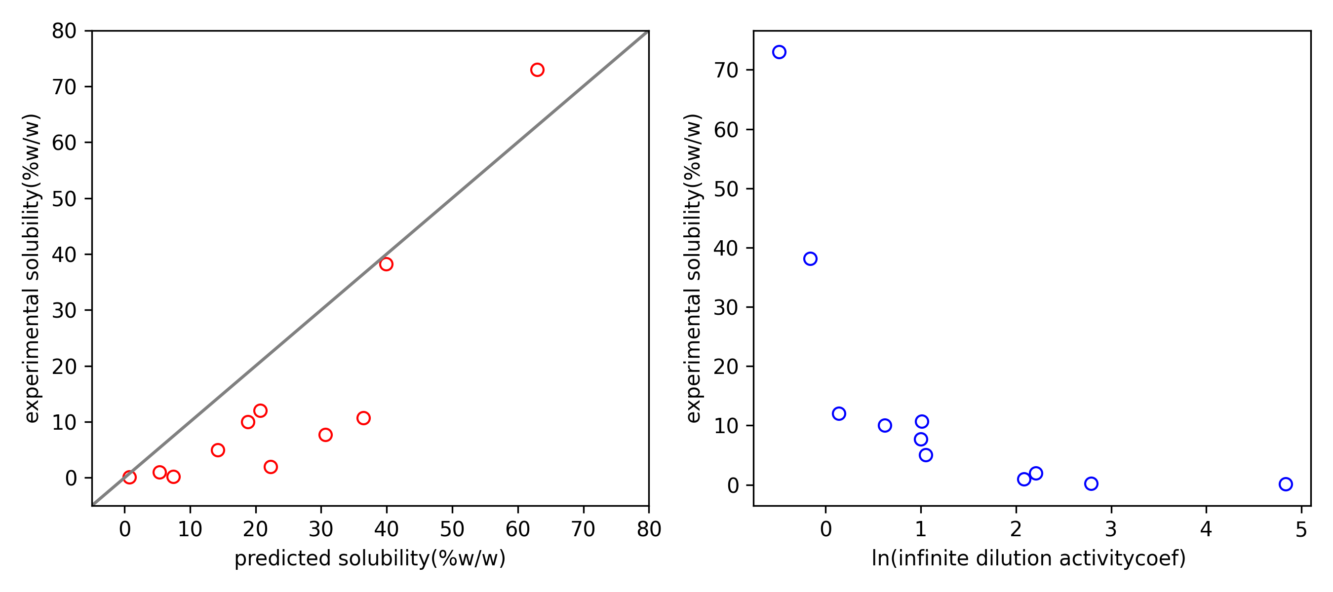
Fig. 7 The comparison of experimental solubility with (1) predicted solubility and (2) infinite dilution activity coefficient.

In the second script example, the solubility screening is configured using the set_CRSJob_solubility function within the script. While this approach require appropriately setting up the PLAMS input setting within the function, it provide greater flexibility for configuring unconventional calculations, such as ionic liquids screening.

Python code using PLAMS

[show/hide code]

import os, time
import multiprocessing
import numpy as np
import matplotlib.pyplot as plt
from scm.plams import Settings, init, finish, CRSJob, config, JobRunner

init()

#######  Note: Ensure to download the coskf_solubility before running the script  #######


def set_CRSJob_solubility(index, ncomp, coskf, database_path, cal_type, method, temperature, comp_input={}):

    s = Settings()  # initialize a settings object
    s.input.property._h = cal_type  # specify problem type
    s.input.method = method  # specify method
    s.input.temperature = temperature  # specify temperature

    compounds = [Settings() for i in range(ncomp)]  # initialization of compounds
    for i in range(ncomp):
        compounds[i]._h = os.path.join(database_path, coskf[i])  # specify absolute directory of coskf file
        for column, value in comp_input.items():  # specify compound's information through comp_input, for example
            if value[i] != None:  # column: frac1, meltingpoint, hfusion
                compounds[i][column] = value[i]
    s.input.compound = compounds

    my_job = CRSJob(settings=s)  # create jobs
    my_job.name = cal_type + "_" + str(index)  # specify job name

    return my_job


Parallel_run = True
Plot_option = True

if Parallel_run:
    config.default_jobrunner = JobRunner(
        parallel=True, maxjobs=8
    )  # Set jobrunner to be parallel and specify the numbers of jobs run simutaneously (eg. multiprocessing.cpu_count())
    config.default_jobmanager.settings.hashing = None  # Disable rerun prevention
    config.job.runscript.nproc = 1  # Number of cores for each job
    config.log.stdout = 1  # suppress plams output default=3

###----INPUT YOUR DATA HERE----###

database_path = os.path.join(os.getcwd(), "coskf_solubility")
cal_type = "solubility"
method = "COSMORS"
ncomp = 2
solvents = [
    "Glycerol.coskf",
    "1,2-Propylene_glycol.coskf",
    "Hexadecane.coskf",
    "Ethanol.coskf",
    "Di-n-octyl_ether.coskf",
    "beta-Pinene.coskf",
    "Isopropyl_myristate.coskf",
    "Propylene_carbonate.coskf",
    "Di-2-ethylhexyl-adipate.coskf",
    "Dimethyl-isosorbide.coskf",
    "Dimethoxymethane.coskf",
]
solute = "avobenzone.coskf"

temperature = 298.15  # K

# store input data along with the necessary thermal property in comp_input dictionary
comp_input = {}
comp_input["name"] = ["solvent", "solute"]
comp_input["frac1"] = [1, 0]  # mole fraction
comp_input["meltingpoint"] = [None, 355]  # melting point(K)
comp_input["hfusion"] = [None, 5.565]  # heat of fusion(Kcal/mol)

# Experimental solubility data in %w/w
exp_sol = [0.1, 0.2, 1, 2, 5, 7.7, 10, 10.7, 12, 38.2, 73]

###----INPUT END----###

index = 0
outputs = []
for solv in solvents:
    coskf = [solv, solute]
    job = set_CRSJob_solubility(index, ncomp, coskf, database_path, cal_type, method, temperature, comp_input)
    index = index + 1
    outputs.append(job.run())

print(job.get_input())


# In a parallel run, the get_results function will wait for the completion of the corresponding jobs.
results = []
for out in outputs:
    results.append(out.get_results())

if Plot_option:
    if cal_type == "solubility":

        cal_sol = [res["solubility massfrac"][1][0] * 100 for res in results]
        cal_lnact = [np.log(res["gamma"][1][0]) for res in results]

        plt.figure(figsize=(5, 4))
        plt.plot(cal_sol, exp_sol, "o", color="Red", markerfacecolor="none", label=method)
        plt.plot([-5, 80], [-5, 80], color="gray")
        plt.xlim([-5, 80])
        plt.ylim([-5, 80])
        plt.xlabel("predicted solubility(%w/w)")
        plt.ylabel("experimental solubility(%w/w)")

        plt.tight_layout()
        # plt.savefig('./PLAMS_solubility_screening.png',dpi=300)
        plt.show()

finish()

References

1

Benazzouz, Adrien, et al. “Hansen approach versus COSMO-RS for predicting the solubility of an organic UV filter in cosmetic solvents.” Colloids and Surfaces A: Physicochemical and Engineering Aspects 458 (2014): 101-109.