Interacting Quantum Atoms (IQA)
This tutorial will show you how to perform interacting quantum atoms calculations with two simple examples: water and PF5 . You will run them and check the results in the output files.
As mentioned in the ADF user documentation, this feature is limited to inter-atomic interactions with some restrictions: closed-shell systems only, no parallelization (NSCM=1), no relativistic options and no symmetry allowed (SYMMETRY NoSym). These restrictions will automatically be enforced when using AMSinput to set up your calculation.
Step 1: Build H2O
- Start AMSinputAdd an oxygen atom using O tool then add the hydrogens (ctrl/cmd + E)Choose the Geometry Optimization task in main sectionChoose the DZP basis set, and no frozen coreSet Relativity → NoneSave and Run

At the end of the job:
- Read the new coordinates as suggested.
Step 2: Calculate all inter-atomic interactions in H2O
- Choose the Single Point task in main section (mandatory for an IQA calculation)In the panel bar, select Properties → QTAIMCheck the Calculate Interacting Quantum Atoms (IQA) checkboxSave again and Run

Step 3: Analyze the results
When the calculation has finished, check the results:
- Open the output file: SCM → OutputGo to the IQA section of the output (Properties → Interacting Quantum Atoms (IQA) )

As mentioned in the output, all results are expressed in a.u. unless otherwise specified (kcal/mol). By default, only the total interaction energy as well as the exchange (covalent part) and classical Coulomb electrostatic contributions (ionic part) are listed for each atom pair. In this release, no intra-atomic (‘self’) terms are evaluated.
For instance, the total interaction energy between O1 and H2 atoms corresponds to -287 kcal/mol at this level of theory (LDA/DZP/Normal Grid). The ‘covalent’ part (exchange) is equal to -136 kcal/mol (47% of the total energy) while the electrostatic contribution (‘ionic part’) corresponds to -151 kcal/mol (53% of the total energy).
It is interesting to note that the repulsive H2-H3 interaction is quite large (73 kcal/mol), due to substantial QTAIM charges on hydrogen atoms (+0.55 e- for each hydrogen). The classical Coulomb part of the energy (+ 74 kcal/mol) is larger than the total interaction energy, explaining why the energy percentage is greater than 100%. It is in fact counterbalanced by stabilizing but rather small exchange energy (less than 1 kcal/mol, consistent with the non-bonded character of the interaction). Finally, we can notice that the electrostatic contribution can be roughly estimated by a point charge model (with QTAIM charges) and Coulomb’s law q(H2) x q(H3) / rH2-H3 » 64 kcal/mol.
Step 4: Build PF5
We will now look at the P-F bonds in the PF5 molecule.
- Close all previous windows and start again AMSinputBuild a trigonal bipyramidal structure: Structure Tool → Metal Complexes → ML5 trigonal bipyramidalChange the central atom into a P atomChange ligands into F atomsChoose the Geometry Optimization task in main sectionChoose the DZP basis set, and no frozen coreSet Relativity → NoneSave and Run

At the end of the job:
- Read the new coordinates as suggested.
Step 5: Select two atoms (P and equatorial F) and calculate this specific interaction
- Choose the Single Point task in main section (again, it is mandatory for an IQA calculation)In the panel bar, select Properties → QTAIMCheck the Calculate Interacting Quantum Atoms (IQA) check-boxSelect the central P atom and only one of the equatorial FTo include only these two atoms in the calculation, click the + buttonSelect the verbose modeSave again and Run

Step 6: Analyze the results (a single P-Feq bond in PF5 )
When the calculation has finished, check the results:
- Open the output file: SCM → OutputSearch for the IQA section
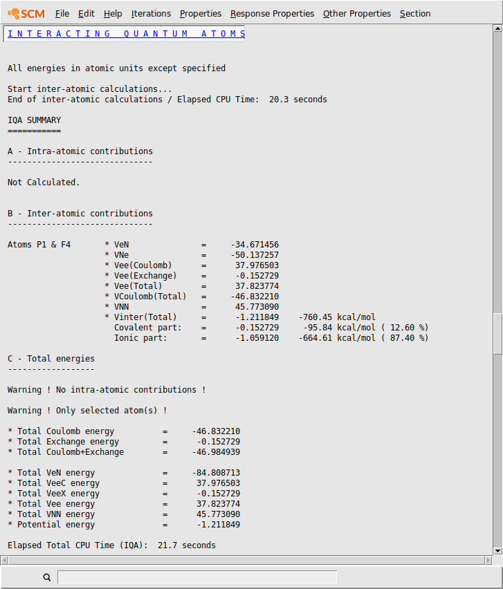
In this verbose mode, more information is printed. Each term is are self-explanatory (see documentation for more information). A third section is added (total energies). In the present release, the various energy contributions are summed up and listed, keeping in mind that ‘self’ contributions are missing. Moreover, this calculation is limited to a single inter-atomic interaction.
Coming back to bonding analysis, the P-Feq bond is predominantly ionic (87%) with a total interaction energy of -760 kcal/mol. Please note that this inter-atomic energy should not be confused with a bond formation energy that includes the variations of intra-atomic terms during the bond formation and substantial secondary interactions between the incoming fluorine atom and other fluorine atoms.
Step 7: Compare equatorial and axial P-F bonds
As a final exercise, one can calculate the inter-atomic interaction between the central P atom with one of the axial F atoms.
- Please close all previous results and go back to the AMSinput windowIn the panel bar, select Properties → QTAIMClick on the – button to deselect atoms and select again P with one axial F atom.Click on the + button to select them.Save and Run again

At the end of the job, open the output file: SCM -> Output Search for the IQA section.
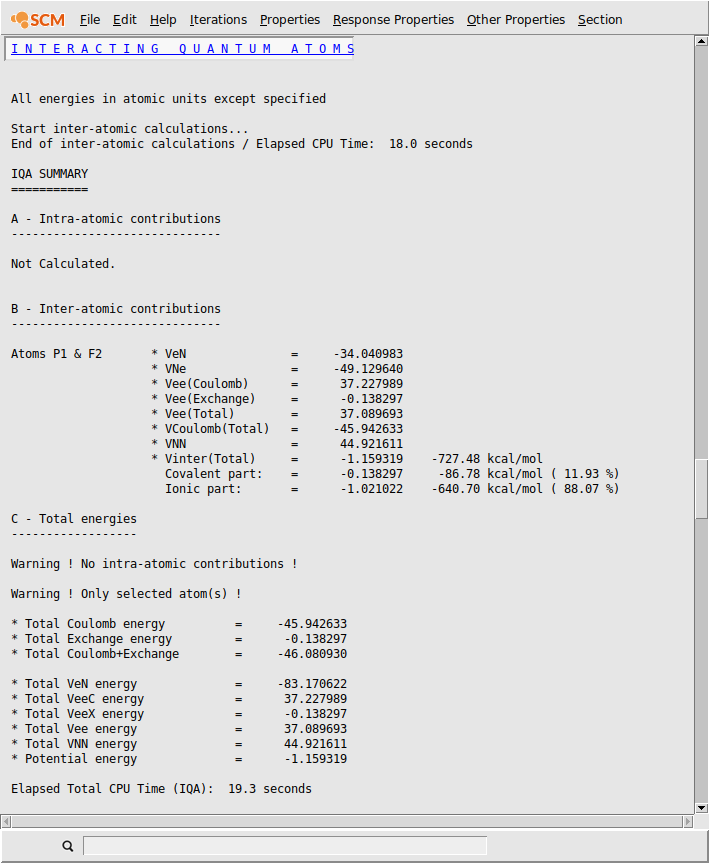
From a pure geometric point of view, the P-Fax bond length is longer than the P-Feq one. Therefore, we may expect a weaker P-Fax bond compared to P-Feq.
The IQA energy decomposition analysis confirms our chemical intuition. Indeed, the covalent contribution to the interaction decreases (from 96 kcal/mol to -87 kcal/mol) as well as the classical Coulomb interaction (from -664 kcal/mol to -640 kcal/mol). This results in a substantial decrease of the total inter-atomic interaction, from -760 kcal/mol to -727 kcal/mol in agreement with the bond length increase.
From a more practical point of view, classical Coulomb interaction energies may be extremely sensitive to the choice of the basis set. This can be seen in the following table (fixed geometry at PBE0/TZ2P; Grid normal):
Xc/Basis           P-Feq                                  P-Fax
                   Ex       Ecoul     Einter              Ex      Ecoul    Einter
PBE0/DZP           -91      -734      -825                -75     -724     -799
PBE0/TZP           -90      -754      -844                -74     -736     -810
PBE0/TZ2P          -86      -792      -878                -72     -769     -841
PBE0/QZ4P          -83      -830      -913                -71     -790     -861
The quality of the integration grid is also important for evaluating this electrostatic contribution. We recommend a “good quality” which seems sufficient. A “normal” level can be used for semi-quantitative purposes. This can be seen in the following table, Geometry & Single Point calculations using PBE0/TZ2P:
Quality           P-Feq                                  P-Fax
                  Ex       Ecoul     Einter              Ex      Ecoul    Einter
Basic             -90       -688      -778               -83     -622     -705
Normal            -86       -792      -878               -72     -769     -841
Good              -82       -831      -913               -70     -784     -854
Excellent         -80       -830      -910               -69     -790     -859