Reaction path and TS search using NEB
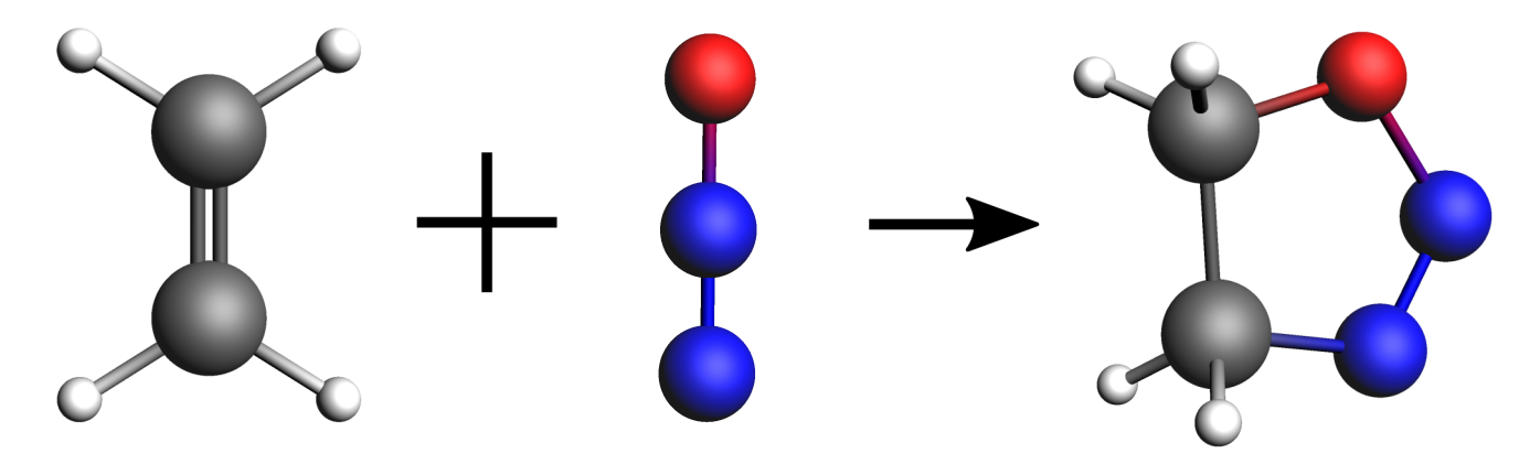
In this tutorial we will use the climbing-image Nudged Elastic Band method (NEB) to find the minimum energy reaction path and transition state of the following reaction:
We will be using the DFTB engine with the GFN1-xTB model. This is a computationally fast method (which is convenient for the purposes of a tutorial) but it is not very accurate in predicting reaction energies. For better accuracy, using the DFT engine ADF (or BAND) is recommended.
Setting up and running the calculation
You can set up and run the calculations for this tutorial using either the Graphical User Interface (GUI), the python library PLAMS or a bash script.
- Start AMSjobs1. in the menu bar select SCM → New input
This will open a new AMSinput window.
- In AMSinput:1. Switch to the DFTB panel:
 →
→  2. Select Task → NEB
We will use the GFN1-xTB model, which is the default model as of the AMS2020 release. Your AMSinput window should look like this:

When setting up an NEB calculation we need to specify two systems: the initial and final states of the reaction. The NEB algorithm will then generate a set of images by interpolating between the initial and final systems. This will be the initial approximation of the reaction path, which will be optimized during the NEB calculation.
- 1. Download the following xyz files: file
NEB_initial.xyzandNEB_final.xyz2. Import the coordinates of the initial system: in the menu bar, select File → Import Coordinates… and select the file NEB_initial.xyz3. Create a new molecule-tab: in the menu bar, select Edit → New Molecule…4. Import the coordinates of the final system in the newly created molecule tab: in the menu bar, select File → Import Coordinates… and select the file NEB_final.xyz
You can switch between the two molecule tabs by clicking on the tabs named Mol-1 and Mol-2 at the bottom of the molecule drawing area.
Important
In NEB calculations, the order of the atoms in the initial and final system should be the same (if you provide an intermediate system, you should use a consistent atom-ordering for that too). The order of the atoms should be consistent because the images-interpolation algorithm maps the n-th atom of the initial system to the n-th atom of the final system.
You can see the indices of the atoms by clicking in the menu bar on View → Atom Info → Name → Show. It is possible to change the order of the atoms in the Coordinates panel (in the panel bar: Model → Coordinates) using the Move atom(s) option.
Now, go to the NEB details panel where we will set up the NEB calculation:
- 1. Click on
 next to Task → NEB to go to the NEB details panel2. From the drop-down menu next to initial system, select Mol-13. From the drop-down menu next to final system, select Mol-24. Check the Characterize PES point checkbox
Your AMSinput window should look like this:

Tip
From most AMSinput panels you can jump to the relevant section of the user manual by clicking on  , which is located in the top-right corner of the panel.
We are now ready to run the calculation:
- In AMSinput:1. In the menu bar, click on File → Save and give it the name “NEB_tutorial”2. In the menu bar, click on File → Run . This will bring the AMSjobs window to the front3. Wait for the calculation to finish. It should take just a few seconds
In the logfile you can monitor the progress of your NEB calculation:
- In AMSjobs:1. Select the job “NEB_tutorial” and in the menu bar click on SCM → Logfile. This will open the logfile
A NEB calculation consists of several steps, which are automatically executed one after the other:
first, the two end points (the initial and final molecules) are optimized (in the logfile, look for
Optimizing initial stateandOptimizing final state)then the NEB reaction path will be optimized (in the logfile, look for
NEB Path Optimization). During the reaction path optimization, the highest-energy image on the path will climb to the transition statefinally, a single point calculation for the TS is performed (in the logfile:
Final calculation for highest-energy image). If the option Characterize PES point is on, then the lowest-lying normal modes will be calculated in order to validate the TS (the TS should have exactly one imaginary frequency). Some information on the reaction path is printed at the end of the logfile:NEB found a transition state! TS barrier height from the left 0.02576078 Hartree 16.165 kcal/mol 67.635 kJ/mol TS barrier height from the right 0.08632064 Hartree 54.167 kcal/mol 226.635 kJ/mol
The following bash script performs an NEB calculation using the AMS driver and the DFTB engine. The input options for the AMS driver described in the AMS driver manual, while the DFTB manual describes the input options for the DFTB Engine block.
#!/bin/sh

"$AMSBIN/ams" << eor

Task NEB

Properties
    PESPointCharacter Yes
End

# The initial system (no header)
System
    Atoms
        N  1.88630912 -0.34204867 -1.59424245
        N  1.14203025 -1.15084766 -1.95458206
        O  0.07639739 -1.27682918 -1.40578886
        C  0.74766633  1.24132374  1.29097263
        C -0.52735637  0.87051548  1.20080269
        H  1.08791192  2.15092371  0.80682956
        H -1.23438622  1.47569873  0.64278673
        H -0.86675778 -0.04061999  1.68265930
        H  1.45534611  0.63457332  1.84647164
    End
End

# The final system should be called 'final'
System final
    Atoms
        N  1.44280525  0.39326405  0.02115802
        N  0.56588608 -0.32983790 -0.53167497
        O -0.68785300 -0.26603404 -0.00725496
        C  0.86550207  1.12517445  1.10513146
        C -0.57889386  0.65549932  1.05974328
        H  0.94852175  2.21696742  0.91684905
        H -1.26384434  1.51200042  0.88137995
        H -0.85746564  0.15513847  2.01191277
        H  1.35845740  0.84559176  2.06071421
    End
End

Engine DFTB
    Model GFN1-xTB
EndEngine
eor
Important
In NEB calculations, the order of the atoms in the initial and final system should be the same (if you provide an intermediate system, you should use a consistent atom-ordering for that too). The order of the atoms should be consistent because the images-interpolation algorithm maps the n-th atom of the initial system to the n-th atom of the final system.
To run the calculation:
- 1. Save the above script in a file called
NEB.run2. Make the script executable: in a terminal, typechmod +x NEB.run3. Run it interactively and redirect the output to a file: in a terminal, type./NEB.run > out
In the following python script (using the PLAMS library) we set up a NEB calculation, run it, and extract some results from the binary results files.
# Load the molecules from file
initial_mol = Molecule('NEB_initial.xyz')
final_mol = Molecule('NEB_final.xyz')

settings = Settings()

# Input options for the AMS driver
settings.input.ams.Task = 'NEB'
settings.input.ams.Properties.PESPointCharacter = 'Yes'

# Input options for the engine (DFTB in this case)
settings.input.DFTB.Model = 'GFN1-xTB'

# You can pass multiple systems to an AMSJob by using a dictionary of molecules.
# The key of the dictionary will be used as the header of the 'System' block
molecules = {'':initial_mol, 'final':final_mol}

# Create and run the job
job = AMSJob(settings=settings, molecule=molecules, name='NEB')
results = job.run()

if job.ok():
    print("Successful NEB calculation!")
    # Collect the results
    pes_point_character = results.readrkf('AMSResults', 'PESPointCharacter', file='NEB_TS_final')
    molecule_ts = results.get_main_molecule()

    # Results on the binary files are in atomic units
    left_barrier = results.readrkf('NEB', 'LeftBarrier')
    right_barrier = results.readrkf('NEB', 'RightBarrier')

    # Convert units using the Units class
    left_barrier_kcalmol = Units.convert(left_barrier,'au','kcal/mol')
    right_barrier_kcalmol = Units.convert(right_barrier,'au','kcal/mol')

    # Print the results
    print(f"PES Point character: {pes_point_character}")
    print("Geometry of the TS:")
    print(molecule_ts)
    print(f"Left TS barrier : {left_barrier_kcalmol:.6f} [kcal/mol]")
    print(f"Right TS barrier: {right_barrier_kcalmol:.6f} [kcal/mol]")
else:
    print("NEB calculation not successful...")
The options for the AMS driver and for the DFTB engine are specified in the Settings object object. The various input keys are described in the AMS driver manual and DFTB manual. See the AMS interface section of the PLAMS manual for more details.
Important
In NEB calculations, the order of the atoms in the initial and final system should be the same (if you provide an intermediate system, you should use a consistent atom-ordering for that too). The order of the atoms should be consistent because the images-interpolation algorithm maps the n-th atom of the initial system to the n-th atom of the final system.
To run the PLAMS script:
- 1. Download the following xyz files:
NEB_initial.xyzandNEB_final.xyz2. Save the above script in a file calledNEB.py3. Run the script using PLAMS: in a terminal, type$AMSBIN/plams NEB.py
To improve the initial approximation of the reaction path in an NEB calculation, you can (optionally) provide an intermediate system.
Another important NEB option is the number of images. In case of problematic NEB path optimization convergence, using more images might help (note that the computation time increases with the number of images used).
You can read more about the various NEB options in the AMS manual.
Results of the calculation
Now, let’s visualize the reaction path computed by NEB:
- In AMSjobs:1. Select the job “NEB_tutorial” and, in the menu bar, click on SCM → Movie. This will open the AMSmovie module

In AMSmovie, you can click on play (or drag the slide-bar) so see the reaction happening. On right-hand side, the energy and gradients of the images in the NEB reaction path are plotted.
The transition state is characterized by having one imaginary frequency. Let’s visualize the normal modes of the transition state geometry with AMSspectra:
- In AMSmovie:1. click on SCM → Spectra. This will open the AMSspectra

Here you will see the computed normal modes for the TS geometry. Notice that there is one negative frequency (imaginary frequency are shown as negative numbers).
- In AMSspectra:1. In the table, click on the line with the negative frequency
The corresponding normal mode will be displayed in the molecule-visualization area. This normal mode gives you an idea of how the atoms are moving as they cross the transition state.
In the folder where you executed your script you will find a file out, which contains the text-output of the calculation, and a folder called ams.results containing binary results of the calculation.
At the end of the output file out you will find a section summarizing the results of the NEB calculation:
NEB found a transition state!


------------------------------------------------------------
TS barrier height from the left         0.02576078 Hartree
                                       16.165 kcal/mol
                                       67.635 kJ/mol
TS barrier height from the right        0.08632064 Hartree
                                       54.167 kcal/mol
                                      226.635 kJ/mol
------------------------------------------------------------
        Transition state geometry

--------
Geometry
--------

Atoms
Index Symbol   x (angstrom)   y (angstrom)   z (angstrom)
   1      N     1.76794468     0.02199401    -0.76530642
   2      N     0.86568320    -0.56021023    -1.14090273
   3      O    -0.28459962    -0.76023024    -0.92163051
   4      C     0.89983351     0.97770099     0.84893165
   5      C    -0.38912967     0.55813520     0.80607959
   6      H     1.18303105     1.94163319     0.44757192
   7      H    -1.15509240     1.14579400     0.31965225
   8      H    -0.73127815    -0.27639812     1.40152984
   9      H     1.61076814     0.51427067     1.51998360
The folder ams.results contains:
- a text file called
ams.logcontaining a very concise summary of the calculation’s progress during the run. - the main binary results file
ams.rkf, containing the reaction path computed in the NEB calculation. - the engine results file
NEB_TS_final.rkfcorresponding a single point calculation at the transition state geometry. It contains, among other properties, the normal modes.
You can explore the content of the rkf binary results files using the kfbrowser utility.
- In a terminal, type:
$AMSBIN/kfbrowser ams.results/NEB_TS_final.rkf
The binary results of the calculation can also be visualized with the GUI modules:
- In a terminal, type:
$AMSBIN/amsmovie ams.results/ams.rkfIn a terminal, type:$AMSBIN/amsspectra ams.results/NEB_TS_final.rkf
This is the output printed by the PLAMS script:
[16:08:17] PLAMS working folder: /home/workdir/plams_workdir
[16:08:17] JOB NEB STARTED
[16:08:18] JOB NEB RUNNING
[16:08:20] JOB NEB FINISHED
[16:08:20] JOB NEB SUCCESSFUL
PES Point character: transition state
Geometry of the transition state:
  Atoms:
    1         N      1.767944      0.021994     -0.765307
    2         N      0.865684     -0.560210     -1.140903
    3         O     -0.284600     -0.760230     -0.921631
    4         C      0.899834      0.977701      0.848932
    5         C     -0.389130      0.558135      0.806080
    6         H      1.183031      1.941633      0.447572
    7         H     -1.155092      1.145794      0.319652
    8         H     -0.731278     -0.276398      1.401530
    9         H      1.610768      0.514271      1.519984

Left  TS barrier: 0.025761 [Hartree]
Right TS barrier: 0.086321 [Hartree]
[16:08:20] PLAMS run finished. Goodbye
In the folder where you executed your script you will find a newly created folder plams_workdir containing the results of the calculations. The folder plams_workdir/NEB contains the results of the job NEB. Inside this folder you will find all the files generated by AMS, including the binary results files ams.rkf and NEB_TS_final.rkf.
The binary results of the calculation can also be visualized with the GUI modules:
- In a terminal, type:
$AMSBIN/amsmovie plams_workdir/NEB/ams.rkfIn a terminal, type:$AMSBIN/amsspectra plams_workdir/NEB/NEB_TS_final.rkf