TDDFT Study of 3 different Dihydroxyanthraquinones¶

For this tutorial we want to answer both scientific questions about the UV/Vis spectra of three different Dihydroxyanthraquinones as well as questions related to the model.

Scientific Questions¶

Q1 When looking at 3 different Dihydroxyanthraquinones, does the position of the hydroxyl groups influence the charge transfer occurring when these molecules are exposed to UVvis light?

Q2 Which vertical electron transfers are responsible for the absorptions in the blue region of the UVvis spectra?

Model Questions¶

AMS offers 4 options of TDDFT, which one is best suited for the problem at hand?

TDDFT

The standard method for excitations in ADF
Works for LDA, GGA, hybrids, range-separated hybrids
It can do an excited state geometry optimization for LDA, GGA, and hybrids, but not for range separated hybrids

TDDFTB

fast standard method for excitations in DFTB
excited state geometry optimizations are possible

TDDFT+TB

excitation method using DFT orbitals from ADF, kernel from DFTB
only for LDA+GGA especially useful if many excitations are required, then much faster than standard
excited state geometry optimization not possible

sTDDFT

excitation method using DFT orbitals from ADF, kernel from DFTB
only for hybrids (and with special parameters for range separated hybrids)
especially useful if many excitations are required, then much faster than standard TDDFT for hybrids
excited state geometry optimization not possible

Prerequisites¶

You should be comfortable drawing a structure, setting up a calculation when given hints, running it, and retrieving results. If not, you can refresh your GUI skills here.

Note

We recommend to do the geometry optimizations and TDDFT calculation on a bigger machine than a PC or laptop as we will use a large basis set.

Overview¶

We will first have to validate our method as we have to show our peers that our choices indeed can deliver credible answers. TDDFT is mentioned very often in the literature and the description in the ADF manual refers to it as a standard method. This makes it a good candidate for a first attempt.

We want to see how good ADF can predict the absorption maxima in the UVvis spectra of 1,4-, 1,5- and 1,8- Dihydroxyanthraquinone (DHAQ) For this we’ll use experimental spectra reported by Zhang et al [1]. These compounds work as photo-initiating systems and show absorption maxima in the blue light wavelength range, which makes them potential candidates to work under the irradiation of blue LED bulbs.

The spectra have been recorded in Acetonitrile which means we have to think about why/if this is important for our calculations – we may have to include solvent effects in our calculations as well. We will talk about this in detail below. We also will only study the absorption in the violet/blue range of the UVvis spectrum, i.e. 380 -485 nm.

It is always a good idea to make a short note of what information we have. We know about the structures, their symmetry and experimental UVvis results.

Symmetry can help us to understand which electron transitions are allowed, as transitions between states of the same parity are forbidden. (Laporte Rule). So, by knowing beforehand what the symmetry of a molecule is we can look at the character table of a point group and work it out.

A proper comparison with experimental spectra would require the inclusion of vibronic effects and a very accurate description of the solvent effects. TDDFT does not cater for vibronic effects and the solvent model we are going to use is an implicit one and describes solvent effects via a dielectric continuum (see COSMO). Also, the quality of the obtained results is profoundly functional-dependent and there is no systematic way to check for improvement. This means we often have to find for each compound family the optimal functional.

Note

Even with the optimal functionals, a mean absolute deviation smaller than 0.25 eV should be considered a good result.

Our DHAQ structures will most likely show n → π * and π → π * transitions as we have an aromatic system with four oxygen atoms. There also will be intramolecular charge-transfer absorption as we have groups with both electron donating and -accepting properties.

Solvents do affect exited species, and peaks resulting from n → π * transitions are shifted to shorter wavelengths (blue/hypsochromic shift). With increasing solvent polarity increased solvation of the lone pair occurs, which lowers the energy of the n orbital. Often (not always), a red/bathochromic shift is seen for π → π * due to attractive polarization forces which lower the energy levels of both the excited and non-excited states.

0. What functional, What basis set?¶

A good starting point is to follow the best-practice advice in SCM’s FAQ section. Further aid can be found in the many overview articles published on TDDFT, e.g.

D. Jacquemin, V. Wathelet, E.A. Perpete, and C. Adamo, Extensive TD-DFT Benchmark: Singlet-Excited States of Organic Molecules, J. Chem. Theory Comput. 2009, 5, 2420–2435

D. Jacquemin, E.A. Perpete, G.E. Scuseria, I.Ciofini, and C. Adamo TD-DFT Performance for the Visible Absorption Spectra of Organic Dyes: Conventional versus Long-Range Hybrids, J. Chem. Theory Comput. 2008, 4, 123-135

1. Geometry Optimization¶

To optimize all three DHAQ isomers use the following workflow. Make sure to choose sensible names for your files such as 14_DHAQ_opt.ams and 14_DHAQ_f.ams so you easily recognize the structure and the sort of computation you did.

: Build each molecule as shown in the table above and make sure the OH do form intramolecular hydrogen bonds with the C=O group. (It is convenient to start from the anthracene geometry, which you can import from the molecule database by clicking the magnifying glass on the top right and typing “anthracene”.)

Symmetrize the molecule by clicking on .

Do not worry if your molecule does not quite have the correct symmetry yet. The geometry optimization will take care of making it symmetric enough, so that it will become perfectly symmetric when we later run the symmetrizer again.

To setup the geometry optimization:

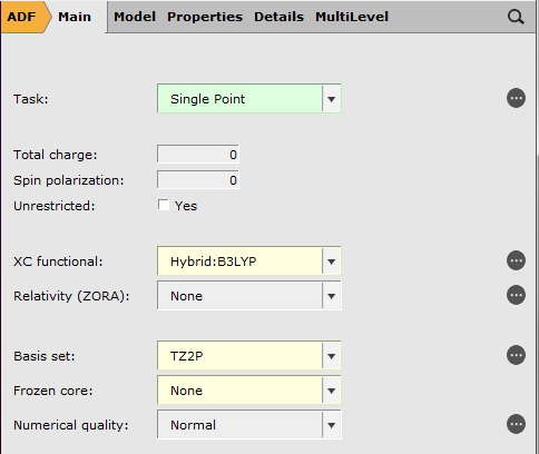
: In the Main tab chose

Task → Geometry Optimization

XC-Functional → Hybrid → B3LYP

Basis set → TZ2P

Frozen Core → None

: Move to the Model tab chose

Solvation → Solvation method → COSMO

COSMO Solvent → Acetonitrile

Tip

To validate that the geometry optimization reached a minimum on the potential energy surface, you can optionally request a PES point characterization:

: In the panel bar, select Properties → IR (Frequencies, VCD)

Check the Characterize PES point check-box

In the text output (or logfile) you can see the results of the PES point characterization

: Save and run the calculation

Once the calculation has finished, you can proceed to the TDDFT calculations. Repeat this for all of your 3 DHAQ structures.

2. TDDFT Calculations¶

To run a TDDFT calculation, make sure you are using the optimized geometries from the previous step.

: In the Main tab chose

Task → Single Point

Symmetrize the molecule by clicking on .

: If you requested Characterize PES point in the previous step, un-check the Characterize PES point check-box in the Properties → IR (Frequencies, VCD) panel

: From the Properties tab choose Excications(UV/Vis),CD

Type of Excitations → SingletAndTriplet

Number of Excitations → 10

: Save and run the calculation

3. Analyzing TDDFT Calculations¶

We will discuss this section using the data of 14-DHAQ.

: Open the result file and go to SCM → Spectra

Select: Axes → Horizontal Unit → eV.

You now can explore your spectrum.

You can investigate peaks, see the symmetry of your transition, the absorption energy in eV and which orbitals are contributing. The peak of interest is the one at 2.495 eV. which we will refer to as 2.50 eV in the following.

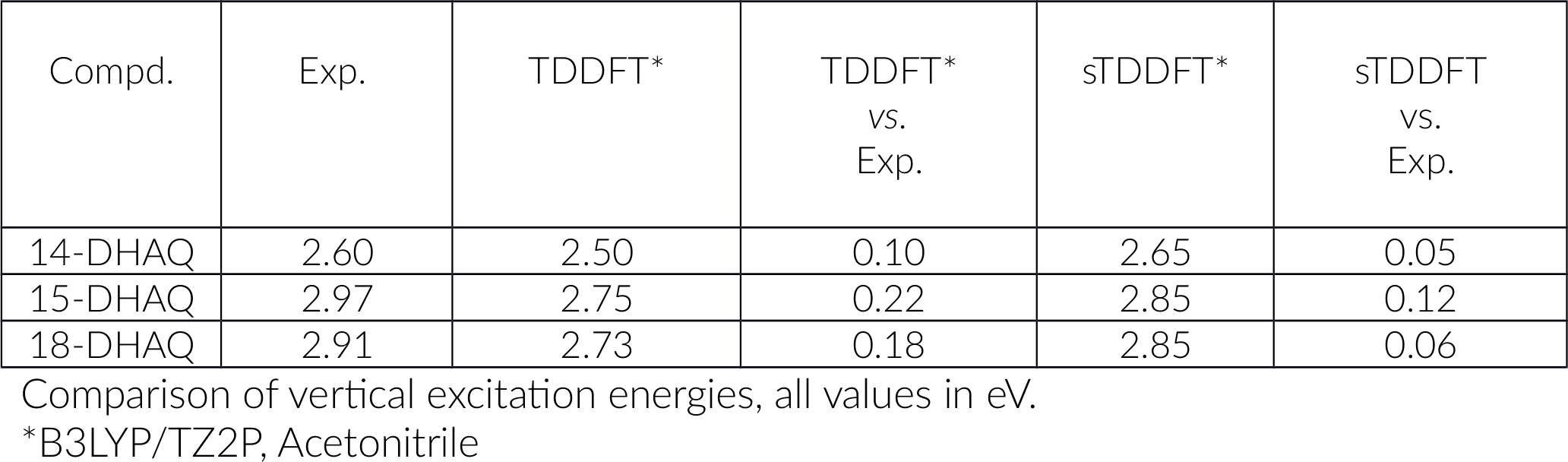
We plan to revisit the actual orbital transition details a bit later. For now, we want to compare our calculations with the experimental data and tabulate the results.

As you can see we got excellent results. Before we move on and discuss the nature of these transitions in detail we want to divert and look into computational effort. You will agree, it did take some time to obtain our results and if we were only interested in these 3 structures it may be ok. However, often we may be confronted with a larger set of structures and some pressure to provide answers fast - and then speed can matter. Thus, we would like the option of a faster method but still have a good accuracy.

4. Faster TDDFT variant: sTDDFT¶

As mentioned in the introduction, the Amsterdam Modeling Suite has several methods that can be used to speed up the calculation of vertical excitation energies. Among others these are

sTDDFT by Bannwarth and Grimme[2]
TDDFT+TB = Uses the molecular orbitals from a DFT ground state calculation as input to an excited state calculation with TDDFTB coupling matrices.
TDDFTB = Time dependent density functional tight-binding.

The acronym sTDDFT stems from “simplified time-dependent density functional theory” and the method allows fast computation of UVvis or circular dichroism (CD) spectra of molecules with 500-1000 atoms.

The method approximates the integrals needed for the exited states calculation and thus needs some parametrization.

Note

For hybrid functionals ADF will automatically set the parameters that are needed in this method. For range-separated functional one needs to set the parameters manually and you need to consult literature to get this right. Symmetry NOSYM is required and a TZP or TZ2P basis set is recommended for this method.

Let us set up the calculations for our 3 DHAQ:

: Starting from the TDDFT calculation in the previous step

go to the Properties tab

choose Excitations(UV/Vis),CD

select Method → sTDDFT

File → Save as, give it a new name and run

: When the calculations are finished, open the result files and go to SCM → Spectra.

Analyze the spectra like before and add to the table.

You can see the results are excellent and we saved a lot of time. How much time the calculation took, can be found in the output file of the calculation.

: Click on the SCM Logo to the left and select Output.

Scroll all the way to the bottom

To show the timings, eg:

Total cpu time:         55.24
Total system time:       3.07
Total elapsed time:     58.83

The timing shows how much time (in seconds) was spent in the ADF code (CPU) and in the kernel (System), and how long did it take for the calculation to complete (Elapsed). You can compare the timing with the TDDFT calculation we ran earlier:

Total cpu time:       1675.52
Total system time:      32.81
Total elapsed time:   1722.08

This means on this particular hardware sTDDFT is 30 times faster than the corresponding TDDFT calculation.

Tip

The speedup and accuracy make the sTDDFT method a good tool for screening excitation energies. If LDA or GGA functionals work for your system and your molecules are large, do try TDDFT+TB. You may follow the workflow described for sTDDFT above, just choose TD- DFT+TB from the “Type of excitations” dropdown menu.

5. Analyzing the Orbitals¶

When we study UVvis absorption properties we want to know which electrons are getting excited and from which occupied orbital they move into which virtual one.

For example, the calculated spectrum of 14-DHAQ was accompanied by some output describing the orbitals involved.

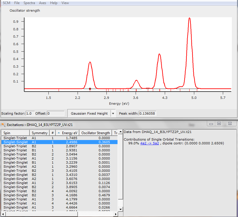
This one is very simple as only one occupied and one virtual molecular orbital (MO) are involved. For 99% the transition from MO 4a2 to MO 5a2 is associated with an excited state and our peak at 2.50 eV.

: Click on 4a2 -> 5a2 to bring up 2 pictures of the orbitals

One of the occupied orbital with red and blue lobes and one of the virtual ones with turquoise and ochre lobes.

Now we need to find out what these MOs are:

: Click on SCM → Levels

In the AMSlevels window opening up, choose View → Labels → Show

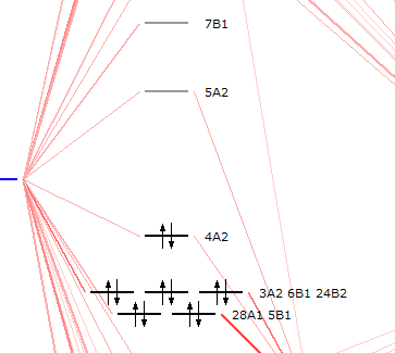
You will see 4A2 is the HOMO and 5A2 is the LUMO. Thus, you know now, that the peak at 2.50 eV is the HOMO-LUMO transfer.

Note

Transitions are not always that simple; you can easily end up with more than a pair of MOs involved and you see nothing but colorful blobs. You can use Natural Transition Orbitals (NTOs). They are usually automatically reported but need some extra persuasion when working with hybrid functionals.

6. Analyzing the NTOs¶

More often you will see in your outputs a list of MOs that contribute equally to an exited state. By transforming all of these MOs (see [3]) to a Natural Transition Orbital (NTO) we can simplify the qualitative description of an electronic transition.

As we are using B3LYP, we require the Tamm-Dancoff Approximation (TDA) before we can do this. TDA has its use for triplet excitations that often lead to instability in the wavefunctions and result in imaginary TDDFT triplet excitation energies.

: Go back to your original TDDFT calculations

tick the box for TDA on the Excitations (UV/Vis),CD panel

save and run

When your calculations are finished

: Open the spectrum again

you will now see an entry for NTO

You will get occupied and virtual NTO in one picture but you can look at them individually by un/checking the boxes next to Isosurface: With Phase.

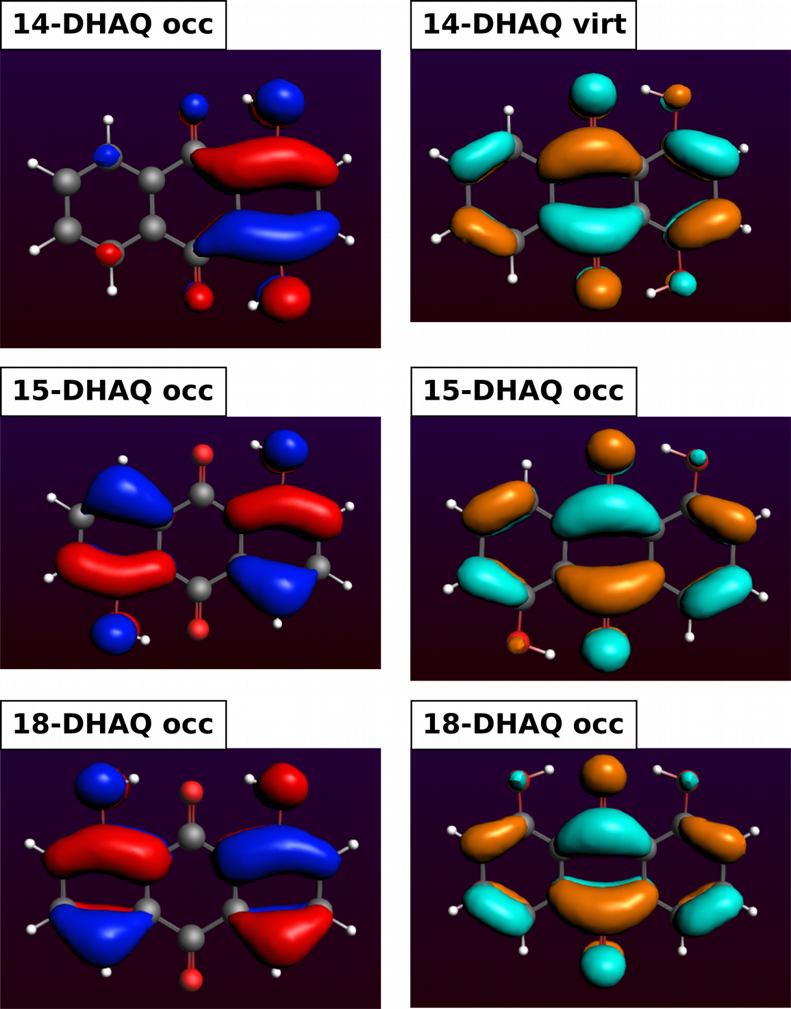
We can see that the lone pairs of the OH oxygen atoms are involved in all DHAQs. In 14-DHAQ the charge is mainly located in the ring carrying both OH groups which is a different behavior. Then we can see for all DHAQs, that the charge transfers to other parts in the molecule and moves to the antibonding C=O orbital, i.e. π*(C=O) but also to some of the π*(C=C).

Thus, can we answer our initial scientific questions?

Q1 When looking at 3 different Dihydroxyanthraquinones, does the position of the hydroxyl groups influences the charge transfer occurring when these molecules are exposed to UVvis light?

A1 Yes, the positions of the OH groups do influence where the charge is located in the ground state. In case of 14-DHAQ it is located mainly at the 6-ring with the two OH groups.

Q2 Which vertical electron transfers are responsible for the absorptions in the blue region of the UVvis spectra?

A2 It’s the HOMO-LUMO transfers and lone pairs of the hydroxyl oxygen atoms are involved and some close-by π(C=C), and as acceptors π*(C=O) but also to π*(C=C) Mos.

7. Localized Analysis of Canonical Molecular Orbitals (CMO) with NBO6¶

Note

This part requires you to have a license for the NBO6 program. You can contact license@scm.com for more information.

Natural Bond Orbitals (http://nbo6.chem.wisc.edu/) can aid to provide a direct link to familiar valency and bonding concepts, similar to what we used from Lewis Structures.

Here in particular, we are interested in the CMO analysis, which allows us to tabulate the leading NBO contributions (bonding, nonbonding, or antibonding) to each canonical MO. Let’s try it and discuss it as we go along.

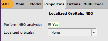
: Open the optimized structure of your 14-DHAQ

Go to Details → Symmetry and select Symmetry → NOSYM

Go to Properties → Localized Orbitals → NBO

Tick Perform NBO analysis: Yes

: Go to Details → Run Script

Uncheck the checkbox Auto Update

We had to disable the use of symmetry earlier, as it is not supported by the NBO program. We do require the Fock matrix to be written out because we need it for our CMO analysis. This is a non-standard feature that can be requested directly in the run script.

: Scroll all the way to the bottom

Add the highlighted keywords to the run file:

# ============
# NBO Analysis
# ============

"$AMSBIN/adfnbo" <<eor
write
fock
spherical
nbo-analysis
eor

"$AMSBIN/gennbo6" FILE47

"$AMSBIN/adfnbo" <<eor
spherical
fock
read
eor

Once it finished you have to go into the result directory of the job and use a text editor (notepad, vi, emacs, nano, etc.) to open the file FILE47 you will find there. You see below the header of this file.

: Replace the highlighted text

$GENNBO NATOMS=  26 NBAS= 556 BOHR BODM $END
$NBO BNDIDX NBONLMO=W AONBO=W AONLMO=W NLMOMO=W STERIC FILE=adfnbo DIST $END
$COORD
****** (NO TITLE) ***

: with the following text

$GENNBO NATOMS=  26 NBAS= 556 BOHR BODM $END
$NBO CMO FILE=adfnbo $END
$COORD
****** (NO TITLE) ***

: Save this file as FILE47_2

Open a terminal (on windows do this)

run the following command

$AMSBIN/gennbo6 FILE47_2 > cmo_output

Once the calculation is finished do open cmo_output and scroll to “CMO: NBO Analysis of Canonical Molecular Orbitals”. Find MO 62 (occ) which is your HOMO. We find:

MO  62 (occ): orbital energy =  ­0.092955 a.u.
               0.499*[ 50]: BD ( 2) C 9­ C10
               ­0.499*[ 46]: BD ( 2) C 7­ C 8
               ­0.369*[ 24]: LP ( 2) O25(lp)
               0.369*[ 20]: LP ( 2) O23(lp)
               0.309*[ 76]: BD*( 2) C 5­ C 6*

We find in square brackets [ ] the number of the NBO and BD stands for bond, CR for core, LP for lonepair and RY for Rydberg. BD* stands for anti-bonding and you may wonder now how the HOMO can be anti-bonding. NBO number [76] is not the same as a virtual MO. It just means some non-Lewis BD* character is weakly mixed in here. You will find the opposite for our LUMO: some Lewis-type BD [56] and [53] is mixing in here:

MO  63 (vir): orbital energy =  ­0.035824 a.u.
               0.472*[ 70]: BD*( 2) C 2­ O24*
               ­0.472*[ 66]: BD*( 2) C 1­ O26*
               0.366*[ 76]: BD*( 2) C 5­ C 6*
               ­0.304*[ 72]: BD*( 2) C 3­ C 4*
               0.264*[ 86]: BD*( 2) C 9­ C10*
               ­0.264*[ 82]: BD*( 2) C 7­ C 8*
               0.235*[ 56]: BD ( 2) C12­ C14
               ­0.235*[ 53]: BD ( 2) C11­ C13

Note

To get the % of the contributions of each NBO you take the square of the preceding numbers times 100, e.g. 0.472 2 x 100.

Next we want to visualize this NBOs in the AMSView:

: Select the NBO job in the AMSJobs and select SCM → View

Add Isosurface: With Phase

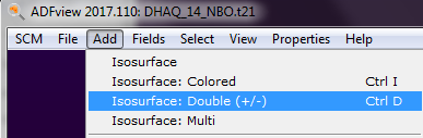
: At the bottom of the window click on Select Field → NBOs

: You will get a Select NBO window and now you have to select one by one the

numbers you found in your CMO results.

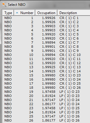
For the HOMO we find

For the LUMO we find

Now we can state the charge transfers from 50% of the π orbitals of the C=C bonds adjacent to the two OH groups and from 28% of the lone pairs of the two hydroxyl towards 48% of the π* orbitals of the C=O bonds and the rest of it settles in π* orbitals of C=C bonds, but never reaches quite as far as the most distant C=C bond of the furthest aromatic ring with respect to the di-hydroxyl moiety.

Lit.:

[1] J. Zhang, J. Lalevée, J. Zhao, B. Graff, M. H. Stenzel and P. Xiao Dihydroxyanthraquinone derivatives: natural dyes as blue-light-sensitive versatile photoinitiators of photopolymerization, Polym. Chem. 7, 7316 (2016).

[2] C. Bannwarth and S. Grimme, A simplified time-dependent density functional theory approach for electronic ultraviolet and circular dichroism spectra of very large molecules, Computational and Theoretical Chemistry, 1040–1041 (2014) 45-53 .

[3] R.L. Martin, Natural transition orbitals, J. Chem. Phys. 118 (2003) 4775-7 .