Li-Ion Diffusion Coefficients in cathode materials
In this tutorial we will compute the diffusion coefficients of Lithium atoms in a Li0.4S cathode by means of molecular dynamics simulations with the ReaxFF engine.
The systems and workflows presented here are originally described in the publication ReaxFF molecular dynamics simulations on lithiated sulfur cathode materials Phys. Chem. Chem. Phys. 17, 3383-3393 (2015).
The tutorial consists of the following steps:
- Importing a CIF file
- Manipulating the structure (e.g. inserting particles) and equilibrating the system
- Creating an amorphous structure by simulated annealing
- Calculating diffusion coefficients from MD trajectories
If you wish, you can download the already-relaxed amorphous Li0.4S structure by clicking here and skip the simulated annealing and equilibration calculations.
Importing the Sulfur(α) crystal structure
- 1. Open a new AMSinput window2. Switch to ReaxFF:
 →
→ 
To speed up the calculations, we will use a smaller system than the one described in the publication. The crystal structure can be directly imported from a CIF file:
- 1. Download the
CIF file by clicking here2. In AMSinput: File → Import Coordinates3. Select the CIF file you just downloaded using the file dialog window
Generating the Li0.4S system
We first need an xyz file of a single Lithium atom:
- 1. Open a new AMSinput: SCM → New Input2. Draw a single Li atom3. File → Export coordinates → .xyz and give it the name “Li.xyz”4. Close the AMSinput window without saving
We use the builder functionality of AMSinput to randomly insert 51 Li-atoms into our Sulfur system.
See also
A better way of building the Li0.4S system is to use Gran Canonical Monte Carlo (GCMC). See also the Battery discharge voltage profiles using Grand Canonical Monte Carlo tutorial.
- 1. Click on Edit → Builder2. Next to “Fill box with”, set the number to 513. Click on the folder and select the “Li.xyz” you just made4. Set Distance to 1.0 Å5. Click on Generate Molecules6. Click on Close

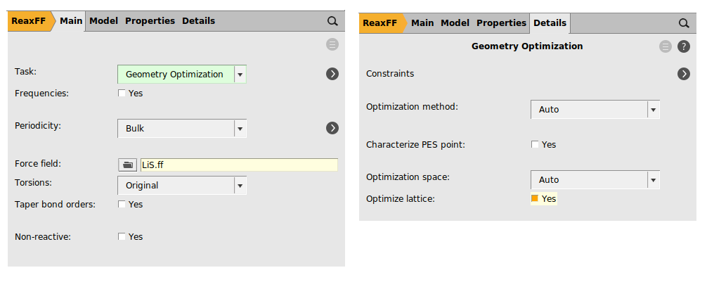
We now need to relax the geometry by running a geometry optimization including lattice relaxation:
- 1. In the main panel, select Task → Geometry Optimization2. Click on the folder next to Force Field and select LiS.ff3. Details → Geometry Optimization4. Tick the Optimize lattice checkbox
We are now ready to run the Li0.4S relaxation calculation:
- 1. File → Save As… and give it an appropriate name (e.g. “LiS_optimization”)2. File → Run3. Click yes when asked if the structure in AMSinput should be updated
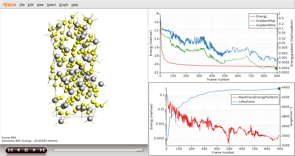
The volume of the unit cell should have increased significantly during the optimization (from about 3300 Å3 to about 4400 Å3):
- 1. Open AMSmovie by clicking on SCM → Movie2. In AMSmovie, click on Graph → Cell volume3. Click on play to see the movie of the geometry optimization
Creating the amorphous systems by simulated annealing
Amorphous systems can be created with a Molecular Dynamics simulation by slowly heating up the system followed by a rapid cool-down.
As in the publication, we will anneal up to 1600 K followed by a rapid cool-down to room temperature. In order to speed up the calculation, only 30000 steps are calculated here.
- 1. In the main panel, select Task → Molecular Dynamics2. Click on
 next to Task: Molecular Dynamics to go to the MD details3. Set the number of steps to 30000

We will now set up the following temperature profile:
- From start until step 5000: T = 300 K (constant)
- From step 5000 to step 25000: heating up from 300 K to 1600 K
- From step 25000 to step 30000: cooling down from 1600 K to 300 K
For more details on temperatures and pressure regimes, see the AMS manual on MD.
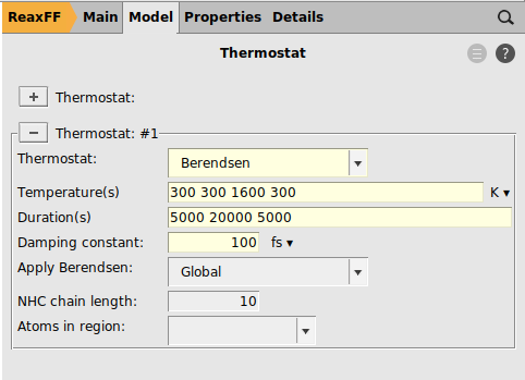
- 1. Click on next to Thermostat to go to the thermostat details2. Click on
 to add a new thermostat3. Select Thermostat → Berensden4. In Temperature(s), set the values
300 300 1600 3005. In Duration(s), set the values5000 20000 50006. Set the damping constant to 100 fs
We are now ready to run the Li0.4S simulated annealing calculation:
- 1. File → Save As… and give it an appropriate name (e.g. “LiS_simulated_annealing”)2. File → Run3. Click yes when asked if the structure in AMSinput should be updated
In AMSmovie you can follow the progress of the MD simulation, and you’ll be able to see the three temperature regimes:
- 1. Open AMSmovie by clicking on SCM → Movie2. In AMSmovie, click on MD Properties → Temperature3. Click on play to see the movie of the MD simulation

We now need to relax the geometry of our new amorphous system by running a geometry optimization including lattice relaxation (as we did before):
- 1. In the main panel, select Task → Geometry Optimization2. Details → Geometry Optimization3. Tick the Optimize lattice checkbox4. File → Save As… and give it an appropriate name (e.g. “LiS_amorphous_optimization”)5. Run the calculation6. Click yes when asked if the structure in AMSinput should be updated
Calculating the diffusion coefficients
We are now ready to run the final MD simulation to compute the Lithium diffusion coefficient at T=1600 K.
AMS calculates the diffusion coefficient by integration of the velocity autocorrelation function:
To compute \(D\) accurately in this way, it is necessary to frequently write the atomic velocities to the trajectory file.
We will use a minimal proof-of-principle setup of 10000 equilibration steps followed by only 100000 production steps:
- 1. In the main panel, select Task → Molecular Dynamics2. Click on next to Task: Molecular Dynamics to go to the MD details3. Set the number of steps to 1100004. Set the Sample frequency to 5 (this writes both the atomic positions and velocities to disk every 5 steps)5. Click on next to Thermostat to go to the thermostat details6. Set the Temperature to 1600 K7. Clear the Duration field8. Set the damping constant to 100 fs
We are now ready to run the calculation:
- 1. File → Save As… and give it an appropriate name (e.g. “LiS_MD_1600K”)2. File → Run3. You can follow the progress of the calculation in AMSMovie and AMStail (SCM → Logfile)
After the calculation is finished, we can obtain the Li diffusion coefficient by computing the velocity autocorrelation function for the Li atoms:
- 1. In AMSMovie select MD Properties → Autocorrelation function2. In Steps set 2000 - 220013. Select Properties → Diffusion Coefficient (D)4. In the visualization area, select one of the Li atoms, and then Select → Select atoms of the same type5. With all Lithium atoms selected, click on next to Atoms: in the Autocorrelation Function panel6. Click on Generate ACF
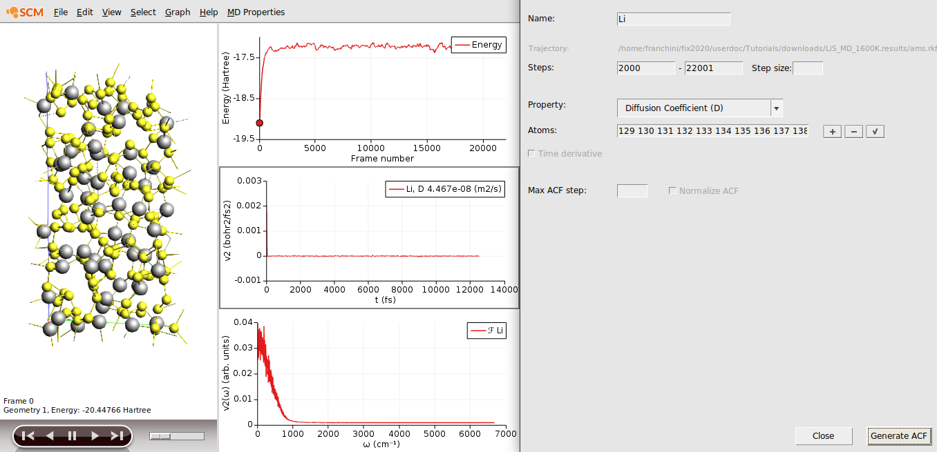
The value of the Diffusion Coefficient D for the Li atoms is \(4.5 \times 10^{-8}\) m2/s (since we are not running a very long MD simulations, you might obtain a slightly different value).
Calculating the diffusion coefficient at 300K would require a very long trajectory. However, it is possible to provide an upper bound to the Li diffusion by means of extrapolation from elevated temperatures using the Arrhenius equation:
where \(D_0\) is the pre-exponential factor, \(E_a\) is the activation energy, \(k_B\) is the Boltzmann constant, and \(T\) is the temperature. The activation energy and pre-exponential factors can then be obtained from an Arrhenius plot of \(\ln{(D(T))}\) against \(1/T\). In order to extrapolate the diffusion coefficients for Li0.4S we calculate trajectories for at least four different temperatures (600 K, 800 K, 1200 K, 1600 K) for each system. One can then extrapolate the diffusion coefficient to lower temperature.