Engine ASE with Import and File Calculators¶

Run the ASE engine from Python in two common ways: with an imported ASE calculator for the EMT quickstart, and with a calculator loaded from a Python file for a custom zero-force example.

Downloads: Notebook | Script ?

Requires: AMS2026 or later

Engine ASE with Import and File Calculators¶

This example shows two ways to run the ASE engine from Python with a ChemicalSystem. First, it reproduces the ASE quickstart with the EMT calculator using Type Import. Then it uses a Python file (Type File) for a custom calculator.

Import the modules¶

We use ChemicalSystem for the structure, Settings to define the AMS input, and view to inspect systems.

from pathlib import Path
import os

from scm.base import ChemicalSystem
from scm.plams import AMSJob, Settings, view

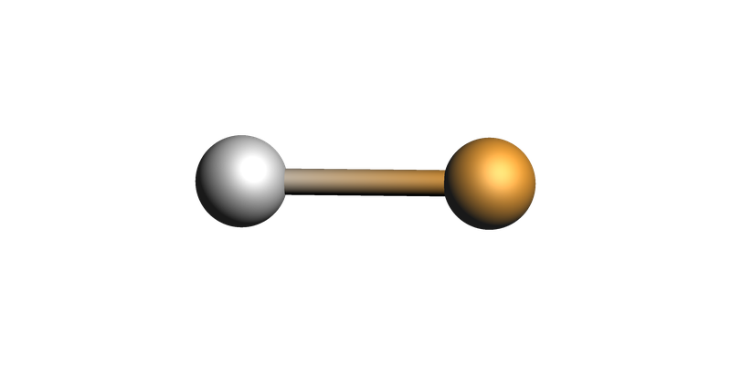
Create the Ag-Cu test system¶

This matches the ASE quickstart example from the manual.

quickstart_system = ChemicalSystem(
    """
System
  Atoms
    Ag 0.0 0.0 0.0
    Cu 0.0 0.0 2.0
  End
End
"""
)
view(quickstart_system, direction="tilt_x", guess_bonds=True)

Run the ASE quickstart with `Type Import`¶

The ASE engine imports ase.calculators.emt.EMT. The extra ASE options are passed with the multiline literal s.input.ASE.Arguments._1 format.

s = Settings()
s.input.ams.Task = "GeometryOptimization"
s.input.ams.Properties.Gradients = "Yes"
s.input.ASE.Type = "Import"
s.input.ASE.Import = "ase.calculators.emt.EMT"
s.input.ASE.Arguments._1 = """
# arguments go here (uncomment the lines)
# arg1 = 3.14
# arg2 = "some value"
"""

quickstart_job = AMSJob(settings=s, molecule=quickstart_system, name="ase_quickstart")
print(quickstart_job.get_input())

Properties
  Gradients Yes
End

Task GeometryOptimization

System
   Atoms
      Ag 0 0 0
      Cu 0 0 2
   End
End

Engine ASE
  Arguments

# arguments go here (uncomment the lines)
# arg1 = 3.14
# arg2 = "some value"

  End
  Import ase.calculators.emt.EMT
  Type Import
EndEngine

quickstart_results = quickstart_job.run()

print(f"Final energy: {quickstart_results.get_energy(unit='eV'):.6f} eV")
print("Final gradients (eV/angstrom):")
print(quickstart_results.get_gradients(energy_unit="eV", dist_unit="angstrom"))

[19.03|09:00:42] JOB ase_quickstart STARTED
[19.03|09:00:42] JOB ase_quickstart RUNNING
[19.03|09:00:43] JOB ase_quickstart FINISHED
[19.03|09:00:43] JOB ase_quickstart SUCCESSFUL
Final energy: 2.746820 eV
Final gradients (eV/angstrom):
[[-0.         -0.          0.00335499]
 [-0.         -0.         -0.00335499]]

quickstart_final_system = quickstart_results.get_main_system()
print("Distance matrix: (angstrom)")
print(quickstart_final_system.distance_matrix())
view(quickstart_final_system, direction="tilt_x", guess_bonds=True)

Distance matrix: (angstrom)
[[0.         2.30152063]
 [2.30152063 0.        ]]

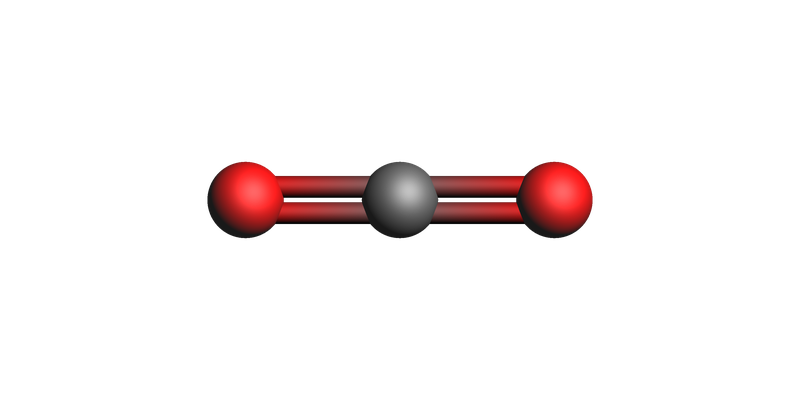
Build the CO$_2$ system for the custom calculator example¶

AMS includes a “zero” ASE calculator defined in the file $AMSHOME/scripting/scm/backends/_zero/calculator.py. The purpose of this section is to illustrate how to specify a file with a custom ASE calculator.

The custom zero calculator always returns zero forces, so the geometry optimization should keep this linear structure unchanged.

zero_system = ChemicalSystem(
    """
System
  Atoms
    O 1.5 0.0 0.0
    C 0.0 0.0 0.0
    O -1.5 0.0 0.0
  End
End
"""
)
view(zero_system, guess_bonds=True)

Run the custom `Zero` example with `Type File`¶

Here the ASE engine loads the calculator from the file distributed with AMS. The calculator argument is again given through the multiline literal format.

If the ASE calculator is installed in a separate conda or uv environment, you can specify that environment using the arguments below.

zero_calculator_file = "$AMSHOME/scripting/scm/external_engines/backends/_zero/calculator.py"

s = Settings()
s.input.ams.Task = "GeometryOptimization"
s.input.ASE.Type = "File"
s.input.ASE.File = zero_calculator_file
s.input.ASE.Arguments._1 = """
energy_per_atom = 1.0
"""
s.input.ASE.Python.Type = "amspython"

# for Conda:
# s.input.ASE.Python.Type = "Conda"
# s.input.ASE.Python.Conda = "name-of-conda-env"

# for uv:
# s.input.ASE.Python.Type = "Uv"
# s.input.ASE.Python.Uv = "/path/to/uv/project"

zero_job = AMSJob(settings=s, molecule=zero_system, name="ase_zero")
print(zero_job.get_input())

Task GeometryOptimization

System
   Atoms
      O 1.5 0 0
      C 0 0 0
      O -1.5 0 0
   End
End

Engine ASE
  Arguments

energy_per_atom = 1.0

  End
  File $AMSHOME/scripting/scm/external_engines/backends/_zero/calculator.py
  Python
    Type amspython
  End
  Type File
EndEngine

zero_results = zero_job.run()

energy_ev = zero_results.get_energy(unit="eV")
expected_energy_ev = len(zero_system) * 1.0

print(f"Final energy: {energy_ev:.6f} eV")
print(f"Expected energy from 1.0 eV per atom: {expected_energy_ev:.6f} eV")
print("Maximum absolute gradient component (eV/angstrom):")
print(abs(zero_results.get_gradients(energy_unit="eV", dist_unit="angstrom")).max())

[19.03|09:00:45] JOB ase_zero STARTED
[19.03|09:00:45] JOB ase_zero RUNNING
[19.03|09:00:46] JOB ase_zero FINISHED
[19.03|09:00:46] JOB ase_zero SUCCESSFUL
Final energy: 3.000000 eV
Expected energy from 1.0 eV per atom: 3.000000 eV
Maximum absolute gradient component (eV/angstrom):
0.0

zero_final_system = zero_results.get_main_system()
print("Distance matrix: (angstrom)")
print(zero_final_system.distance_matrix())
view(zero_final_system, guess_bonds=True)

Distance matrix: (angstrom)
[[0.  1.5 3. ]
 [1.5 0.  1.5]
 [3.  1.5 0. ]]

Python Script¶

#!/usr/bin/env python
# coding: utf-8

# ## Engine ASE with Import and File Calculators
#
# This example shows two ways to run the ASE engine from Python with a `ChemicalSystem`.
# First, it reproduces the ASE quickstart with the EMT calculator using `Type Import`.
# Then it uses a Python file (`Type File`) for a custom calculator.

# ## Import the modules
#
# We use `ChemicalSystem` for the structure, `Settings` to define the AMS input, and `view` to inspect systems.

from pathlib import Path
import os

from scm.base import ChemicalSystem
from scm.plams import AMSJob, Settings, view


# ## Create the Ag-Cu test system
#
# This matches the ASE quickstart example from the manual.

quickstart_system = ChemicalSystem(
    """
System
  Atoms
    Ag 0.0 0.0 0.0
    Cu 0.0 0.0 2.0
  End
End
"""
)
view(quickstart_system, direction="tilt_x", guess_bonds=True, picture_path="picture1.png")


# ## Run the ASE quickstart with `Type Import`
#
# The ASE engine imports `ase.calculators.emt.EMT`. The extra ASE options are passed with the multiline
# literal `s.input.ASE.Arguments._1` format.

s = Settings()
s.input.ams.Task = "GeometryOptimization"
s.input.ams.Properties.Gradients = "Yes"
s.input.ASE.Type = "Import"
s.input.ASE.Import = "ase.calculators.emt.EMT"
s.input.ASE.Arguments._1 = """
# arguments go here (uncomment the lines)
# arg1 = 3.14
# arg2 = "some value"
"""

quickstart_job = AMSJob(settings=s, molecule=quickstart_system, name="ase_quickstart")
print(quickstart_job.get_input())


quickstart_results = quickstart_job.run()

print(f"Final energy: {quickstart_results.get_energy(unit='eV'):.6f} eV")
print("Final gradients (eV/angstrom):")
print(quickstart_results.get_gradients(energy_unit="eV", dist_unit="angstrom"))


quickstart_final_system = quickstart_results.get_main_system()
print("Distance matrix: (angstrom)")
print(quickstart_final_system.distance_matrix())
view(quickstart_final_system, direction="tilt_x", guess_bonds=True, picture_path="picture2.png")


# ## Build the CO$_2$ system for the custom calculator example
#
# AMS includes a "zero" ASE calculator defined in the file `$AMSHOME/scripting/scm/backends/_zero/calculator.py`. The purpose of this section is to illustrate how to specify a file with a custom ASE calculator.
#
# The custom zero calculator always returns zero forces, so the geometry optimization should keep this linear structure unchanged.

zero_system = ChemicalSystem(
    """
System
  Atoms
    O 1.5 0.0 0.0
    C 0.0 0.0 0.0
    O -1.5 0.0 0.0
  End
End
"""
)
view(zero_system, guess_bonds=True, picture_path="picture3.png")


# ## Run the custom `Zero` example with `Type File`
#
# Here the ASE engine loads the calculator from the file distributed with AMS. The calculator argument is again given through
# the multiline literal format.
#
# If the ASE calculator is installed in a separate conda or uv environment, you can specify that environment using the arguments below.

zero_calculator_file = "$AMSHOME/scripting/scm/external_engines/backends/_zero/calculator.py"

s = Settings()
s.input.ams.Task = "GeometryOptimization"
s.input.ASE.Type = "File"
s.input.ASE.File = zero_calculator_file
s.input.ASE.Arguments._1 = """
energy_per_atom = 1.0
"""
s.input.ASE.Python.Type = "amspython"

# for Conda:
# s.input.ASE.Python.Type = "Conda"
# s.input.ASE.Python.Conda = "name-of-conda-env"

# for uv:
# s.input.ASE.Python.Type = "Uv"
# s.input.ASE.Python.Uv = "/path/to/uv/project"

zero_job = AMSJob(settings=s, molecule=zero_system, name="ase_zero")
print(zero_job.get_input())


zero_results = zero_job.run()

energy_ev = zero_results.get_energy(unit="eV")
expected_energy_ev = len(zero_system) * 1.0

print(f"Final energy: {energy_ev:.6f} eV")
print(f"Expected energy from 1.0 eV per atom: {expected_energy_ev:.6f} eV")
print("Maximum absolute gradient component (eV/angstrom):")
print(abs(zero_results.get_gradients(energy_unit="eV", dist_unit="angstrom")).max())


zero_final_system = zero_results.get_main_system()
print("Distance matrix: (angstrom)")
print(zero_final_system.distance_matrix())
view(zero_final_system, guess_bonds=True, picture_path="picture4.png")

Engine ASE with Import and File Calculators¶

Engine ASE with Import and File Calculators¶

Import the modules¶

Create the Ag-Cu test system¶

Run the ASE quickstart with `Type Import`¶

Build the CO\(_2\) system for the custom calculator example¶

Run the custom `Zero` example with `Type File`¶

See also¶

Python Script¶

Engine ASE with Import and File Calculators¶

Engine ASE with Import and File Calculators¶

Import the modules¶

Create the Ag-Cu test system¶

Run the ASE quickstart with Type Import¶

Build the CO\(_2\) system for the custom calculator example¶

Run the custom Zero example with Type File¶

See also¶

Related documentation¶

Python Script¶

Run the ASE quickstart with `Type Import`¶

Run the custom `Zero` example with `Type File`¶