Train an M3GNet Potential with ParAMS
This tutorial shows how to
import energy and forces from a trajectory to construct training and validation sets
split a data set into training and validation sets
set up a ParAMSJob for training an M3GNet ML potential
use the trained potential in a new production simulation
Overview
Import reference data from a short liquid-argon trajectory, split it into training and validation sets, train an M3GNet model with ParAMS, and reuse the deployed model in a production MD job.
from scm.plams import plot_molecule
import scm.plams as plams
from scm.params import ParAMSJob, ResultsImporter
import glob
import matplotlib.pyplot as plt
Initialize PLAMS environment
plams.init()
PLAMS working folder: /path/to/plams_workdir.010
Run a quick reference MD job for liquid Ar
In this example we generate some simple reference data.
If you
already have reference data in the ParAMS .yaml format, then you can skip this step
already have reference data in the ASE .xyz or .db format, you can convert it to the ParAMS .yaml format. See :ref:
convert_params_ase.
molecule = plams.Molecule(numbers=[18], positions=[(0, 0, 0)])
box = plams.packmol(molecule, n_atoms=32, density=1.4, tolerance=3.0)
plot_molecule(box);

reference_engine_settings = plams.Settings()
reference_engine_settings.runscript.nproc = 1
reference_engine_settings.input.ForceField.Type = "UFF"
md_job = plams.AMSNVTJob(
    settings=reference_engine_settings,
    molecule=box,
    name="uff_md",
    nsteps=5000,
    temperature=500,
    writeenginegradients=True,
    samplingfreq=500,
)
md_job.run();
[19.02|16:41:44] JOB uff_md STARTED
[19.02|16:41:44] JOB uff_md RUNNING
[19.02|16:41:46] JOB uff_md FINISHED
[19.02|16:41:46] JOB uff_md SUCCESSFUL
Import reference results with ParAMS ResultsImporter
Here we use the add_trajectory_singlepoints results importer. For more details about usage of the results importers, see the corresponding tutorials.
ri = ResultsImporter(settings={"units": {"energy": "eV", "forces": "eV/angstrom"}})
ri.add_trajectory_singlepoints(md_job.results.rkfpath(), properties=["energy", "forces"])
# feel free to add other trajectories as well:
# ri.add_trajectory_singlepoints(job2.results.rkfpath(), properties=["energy", "forces"])   # etc...
["energy('uff_md_frame001')",
 "energy('uff_md_frame002')",
 "energy('uff_md_frame003')",
 "energy('uff_md_frame004')",
 "energy('uff_md_frame005')",
 "energy('uff_md_frame006')",
 "energy('uff_md_frame007')",
 "energy('uff_md_frame008')",
 "energy('uff_md_frame009')",
 "energy('uff_md_frame010')",
... output trimmed ....
 "forces('uff_md_frame002')",
 "forces('uff_md_frame003')",
 "forces('uff_md_frame004')",
 "forces('uff_md_frame005')",
 "forces('uff_md_frame006')",
 "forces('uff_md_frame007')",
 "forces('uff_md_frame008')",
 "forces('uff_md_frame009')",
 "forces('uff_md_frame010')",
 "forces('uff_md_frame011')"]
Optional: split into training/validation sets
Machine learning potentials in ParAMS can only be trained if there is both a training set and a validation set.
If you do not specify a validation set, the training set will automatically be split into a training and validation set when the parametrization starts.
Here, we will manually split the data set ourselves.
Let’s first print the information in the current ResultsImporter training set:
def print_data_set_summary(data_set, title):
    number_of_entries = len(data_set)
    jobids = data_set.jobids
    number_of_jobids = len(jobids)
    print(f"{title}:")
    print(f"    number of entries: {number_of_entries}")
    print(f"    number of jobids: {number_of_jobids}")
    print(f"    jobids: {jobids}")


print_data_set_summary(ri.data_sets["training_set"], "Original training set")
Original training set:
    number of entries: 22
    number of jobids: 11
    jobids: {'uff_md_frame004', 'uff_md_frame007', 'uff_md_frame003', 'uff_md_frame009', 'uff_md_frame001', 'uff_md_frame010', 'uff_md_frame011', 'uff_md_frame006', 'uff_md_frame005', 'uff_md_frame002', 'uff_md_frame008'}
Above, the number of entries is twice the number of jobids because the energy and forces extractors are separate entries.
The energy and force extractors for a given structure (e.g. frame006) must belong to the same data set. For this reason, when doing the split, we call split_by_jobid
training_set, validation_set = ri.data_sets["training_set"].split_by_jobids(0.8, 0.2, seed=314)
ri.data_sets["training_set"] = training_set
ri.data_sets["validation_set"] = validation_set

print_data_set_summary(ri.data_sets["training_set"], "New training set")
print_data_set_summary(ri.data_sets["validation_set"], "New validation set")
New training set:
    number of entries: 16
    number of jobids: 8
    jobids: {'uff_md_frame004', 'uff_md_frame007', 'uff_md_frame001', 'uff_md_frame010', 'uff_md_frame011', 'uff_md_frame006', 'uff_md_frame005', 'uff_md_frame008'}
New validation set:
    number of entries: 6
    number of jobids: 3
    jobids: {'uff_md_frame009', 'uff_md_frame002', 'uff_md_frame003'}
Store the reference results in ParAMS yaml format
Use ResultsImporter.store() to store all the data in the results importer in the ParAMS .yaml format:
yaml_dir = "yaml_ref_data"
ri.store(yaml_dir, backup=False)

# print the contents of the directory
for x in glob.glob(f"{yaml_dir}/*"):
    print(x)
yaml_ref_data/results_importer_settings.yaml
yaml_ref_data/validation_set.yaml
yaml_ref_data/job_collection_engines.yaml
yaml_ref_data/training_set.yaml
yaml_ref_data/job_collection.yaml
Set up and run a ParAMSJob for training ML Potentials
See the ParAMS MachineLearning documentation for all available input options.
Training the model may take a few minutes.
job = ParAMSJob.from_yaml(yaml_dir)
job.name = "params_training_ml_potential"
job.settings.input.Task = "MachineLearning"
job.settings.input.MachineLearning.CommitteeSize = 1  # train only a single model
job.settings.input.MachineLearning.MaxEpochs = 200
job.settings.input.MachineLearning.LossCoeffs.Energy = 10
job.settings.input.MachineLearning.Backend = "M3GNet"
job.settings.input.MachineLearning.M3GNet.Model = "UniversalPotential"
job.settings.input.MachineLearning.Target.Forces.Enabled = "No"
job.settings.input.MachineLearning.RunAMSAtEnd = "Yes"
job.run();
[19.02|16:41:46] JOB params_training_ml_potential STARTED
[19.02|16:41:47] JOB params_training_ml_potential RUNNING
[19.02|16:43:05] JOB params_training_ml_potential FINISHED
[19.02|16:43:05] JOB params_training_ml_potential SUCCESSFUL
Results of the ML potential training
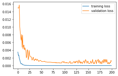
Use job.results.get_running_loss() to get the loss value as a function of epoch:
epoch, training_loss = job.results.get_running_loss(data_set="training_set")
plt.plot(epoch, training_loss)

epoch, validation_loss = job.results.get_running_loss(data_set="validation_set")
plt.plot(epoch, validation_loss)
plt.legend(["training loss", "validation loss"]);
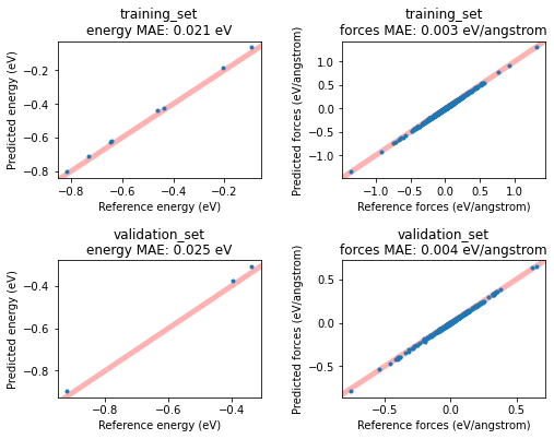
If you set MachineLearning%RunAMSAtEnd (it is on by default), this will run the ML potential through AMS at the end of the fitting procedure, similar to the ParAMS SinglePoint task.
This will give you access to more results, for example the predicted-vs-reference energy and forces for all entries in the training and validation set. Plot them in a scatter plot like this:
fig, axes = plt.subplots(nrows=2, ncols=2, figsize=(8, 6))

for i, data_set in enumerate(["training_set", "validation_set"]):
    for j, key in enumerate(["energy", "forces"]):
        dse = job.results.get_data_set_evaluator(data_set=data_set, source="best")
        data = dse.results[key]
        ax = axes[i][j]
        ax.plot(data.reference_values, data.predictions, ".")
        ax.set_xlabel(f"Reference {key} ({data.unit})")
        ax.set_ylabel(f"Predicted {key} ({data.unit})")
        ax.set_title(f"{data_set}\n{key} MAE: {data.mae:.3f} {data.unit}")
        ax.set_xlim(auto=True)
        ax.autoscale(False)
        ax.plot([-10, 10], [-10, 10], linewidth=5, zorder=-1, alpha=0.3, c="red")

plt.subplots_adjust(hspace=0.6, wspace=0.4);
Get the engine settings for production jobs
First, let’s find the path to where the trained m3gnet model resides using get_deployed_model_paths(). This function returns a list of paths to the trained models. In this case we only trained one model, so we access the first element of the list with [0]:
print(job.results.get_deployed_model_paths()[0])
/path/to/plams_workdir.010/params_training_ml_potential/results/optimization/m3gnet/m3gnet
The above is the path we need to give as the ParameterDir input option in the AMS MLPotential engine. For other backends it might instead be the ParameterFile option.
To get the complete engine settings as a PLAMS Settings object, use the method get_production_engine_settings():
production_engine_settings = job.results.get_production_engine_settings()
print(plams.AMSJob(settings=production_engine_settings).get_input())
Engine MLPotential
  Backend M3GNet
  MLDistanceUnit angstrom
  MLEnergyUnit eV
  Model Custom
  ParameterDir /path/to/plams_workdir.010/params_training_ml_potential/results/optimization/m3gnet/m3gnet
EndEngine
Run a short MD simulation with the trained potential
production_engine_settings.runscript.nproc = 1  # run AMS Driver in serial
new_md_job = plams.AMSNVTJob(
    settings=production_engine_settings,
    molecule=box,
    nsteps=5000,
    temperature=300,
    samplingfreq=100,
    name="production_md",
    timestep=1.0,
)
new_md_job.run(watch=True);
[19.02|16:43:05] JOB production_md STARTED
[19.02|16:43:05] JOB production_md RUNNING
[19.02|16:43:06] production_md: AMS 2024.101  RunTime: Feb19-2024 16:43:06  ShM Nodes: 1  Procs: 1
[19.02|16:43:09] production_md: Starting MD calculation:
[19.02|16:43:09] production_md: --------------------
[19.02|16:43:09] production_md: Molecular Dynamics
[19.02|16:43:09] production_md: --------------------
[19.02|16:43:09] production_md:          Step       Time    Temp.         E Pot        Pressure        Volume
[19.02|16:43:09] production_md:                     (fs)      (K)          (au)           (MPa)         (A^3)
[19.02|16:43:15] production_md:             0       0.00     300.      -0.00672        1048.733        1516.2
... output trimmed ....
[19.02|16:44:15] production_md:          4500    4500.00     335.      -0.03899         524.327        1516.2
[19.02|16:44:16] production_md:          4600    4600.00     363.      -0.04020         523.632        1516.2
[19.02|16:44:17] production_md:          4700    4700.00     361.      -0.03832         541.232        1516.2
[19.02|16:44:18] production_md:          4800    4800.00     335.      -0.03394         592.030        1516.2
[19.02|16:44:20] production_md:          4900    4900.00     279.      -0.02609         687.931        1516.2
[19.02|16:44:21] production_md:          5000    5000.00     359.      -0.03853         551.643        1516.2
[19.02|16:44:21] production_md: MD calculation finished.
[19.02|16:44:22] production_md: NORMAL TERMINATION
[19.02|16:44:22] JOB production_md FINISHED
[19.02|16:44:22] JOB production_md SUCCESSFUL
Open trajectory file in AMSmovie
With the production trajectory you can run analysis tools in AMSmovie, or access them from Python. See the AMS manual for details.
trajectory_file = new_md_job.results.rkfpath()
!amsmovie "{trajectory_file}"
Finish PLAMS
plams.finish()
[19.02|16:44:24] PLAMS run finished. Goodbye
See also
Python Script
#!/usr/bin/env python
# coding: utf-8

# ## Overview
#
# Import reference data from a short liquid-argon trajectory, split it into training and
# validation sets, train an M3GNet model with ParAMS, and reuse the deployed model in a
# production MD job.

from scm.plams import plot_molecule
import scm.plams as plams
from scm.params import ParAMSJob, ResultsImporter
import glob
import matplotlib.pyplot as plt


# ## Initialize PLAMS environment

plams.init()


# ## Run a quick reference MD job for liquid Ar
#
# In this example we generate some simple reference data.
#
# If you
#
# * already have reference data in the ParAMS .yaml format, then you can skip this step
# * already have reference data in the ASE .xyz or .db format, you can convert it to the ParAMS .yaml format. See :ref:`convert_params_ase`.

molecule = plams.Molecule(numbers=[18], positions=[(0, 0, 0)])
box = plams.packmol(molecule, n_atoms=32, density=1.4, tolerance=3.0)
plot_molecule(box)
reference_engine_settings = plams.Settings()
reference_engine_settings.runscript.nproc = 1
reference_engine_settings.input.ForceField.Type = "UFF"
md_job = plams.AMSNVTJob(
    settings=reference_engine_settings,
    molecule=box,
    name="uff_md",
    nsteps=5000,
    temperature=500,
    writeenginegradients=True,
    samplingfreq=500,
)
md_job.run()
# ## Import reference results with ParAMS ResultsImporter
#
# Here we use the ``add_trajectory_singlepoints`` results importer. For more details about usage of the results importers, see the corresponding tutorials.

ri = ResultsImporter(settings={"units": {"energy": "eV", "forces": "eV/angstrom"}})
ri.add_trajectory_singlepoints(md_job.results.rkfpath(), properties=["energy", "forces"])
# feel free to add other trajectories as well:
# ri.add_trajectory_singlepoints(job2.results.rkfpath(), properties=["energy", "forces"])   # etc...


# ## Optional: split into training/validation sets
#
# Machine learning potentials in ParAMS can only be trained if there is both a training set and a validation set.
#
# If you do not specify a validation set, the training set will automatically be split into a training and validation set when the parametrization starts.
#
# Here, we will manually split the data set ourselves.
#
# Let's first print the information in the current ResultsImporter training set:


def print_data_set_summary(data_set, title):
    number_of_entries = len(data_set)
    jobids = data_set.jobids
    number_of_jobids = len(jobids)
    print(f"{title}:")
    print(f"    number of entries: {number_of_entries}")
    print(f"    number of jobids: {number_of_jobids}")
    print(f"    jobids: {jobids}")


print_data_set_summary(ri.data_sets["training_set"], "Original training set")


# Above, the number of entries is twice the number of jobids because the ``energy`` and ``forces`` extractors are separate entries.
#
# The energy and force extractors for a given structure (e.g. frame006) must belong to the same data set. For this reason, when doing the split, we call ``split_by_jobid``

training_set, validation_set = ri.data_sets["training_set"].split_by_jobids(0.8, 0.2, seed=314)
ri.data_sets["training_set"] = training_set
ri.data_sets["validation_set"] = validation_set

print_data_set_summary(ri.data_sets["training_set"], "New training set")
print_data_set_summary(ri.data_sets["validation_set"], "New validation set")


# ## Store the reference results in ParAMS yaml format
#
# Use ``ResultsImporter.store()`` to store all the data in the results importer in the ParAMS .yaml format:

yaml_dir = "yaml_ref_data"
ri.store(yaml_dir, backup=False)

# print the contents of the directory
for x in glob.glob(f"{yaml_dir}/*"):
    print(x)


# ## Set up and run a ParAMSJob for training ML Potentials
#
# See the ParAMS MachineLearning documentation for all available input options.
#
# Training the model may take a few minutes.

job = ParAMSJob.from_yaml(yaml_dir)
job.name = "params_training_ml_potential"
job.settings.input.Task = "MachineLearning"
job.settings.input.MachineLearning.CommitteeSize = 1  # train only a single model
job.settings.input.MachineLearning.MaxEpochs = 200
job.settings.input.MachineLearning.LossCoeffs.Energy = 10
job.settings.input.MachineLearning.Backend = "M3GNet"
job.settings.input.MachineLearning.M3GNet.Model = "UniversalPotential"
job.settings.input.MachineLearning.Target.Forces.Enabled = "No"
job.settings.input.MachineLearning.RunAMSAtEnd = "Yes"


job.run()
# ## Results of the ML potential training
#
# Use ``job.results.get_running_loss()`` to get the loss value as a function of epoch:

epoch, training_loss = job.results.get_running_loss(data_set="training_set")
plt.plot(epoch, training_loss)

epoch, validation_loss = job.results.get_running_loss(data_set="validation_set")
plt.plot(epoch, validation_loss)
plt.legend(["training loss", "validation loss"])
plt.gcf().savefig("picture1.png")
plt.clf()


# If you set ``MachineLearning%RunAMSAtEnd`` (it is on by default), this will run the ML potential through AMS at the end of the fitting procedure, similar to the ParAMS SinglePoint task.
#
# This will give you access to more results, for example the predicted-vs-reference energy and forces for all entries in the training and validation set. Plot them in a scatter plot like this:

fig, axes = plt.subplots(nrows=2, ncols=2, figsize=(8, 6))

for i, data_set in enumerate(["training_set", "validation_set"]):
    for j, key in enumerate(["energy", "forces"]):
        dse = job.results.get_data_set_evaluator(data_set=data_set, source="best")
        data = dse.results[key]
        ax = axes[i][j]
        ax.plot(data.reference_values, data.predictions, ".")
        ax.set_xlabel(f"Reference {key} ({data.unit})")
        ax.set_ylabel(f"Predicted {key} ({data.unit})")
        ax.set_title(f"{data_set}\n{key} MAE: {data.mae:.3f} {data.unit}")
        ax.set_xlim(auto=True)
        ax.autoscale(False)
        ax.plot([-10, 10], [-10, 10], linewidth=5, zorder=-1, alpha=0.3, c="red")

plt.subplots_adjust(hspace=0.6, wspace=0.4)
plt.gcf().savefig("picture2.png")
plt.clf()


# ## Get the engine settings for production jobs
#
# First, let's find the path to where the trained m3gnet model resides using ``get_deployed_model_paths()``. This function returns a list of paths to the trained models. In this case we only trained one model, so we access the first element of the list with ``[0]``:

print(job.results.get_deployed_model_paths()[0])


# The above is the path we need to give as the ``ParameterDir`` input option in the AMS MLPotential engine. For other backends it might instead be the ``ParameterFile`` option.
#
# To get the complete engine settings as a PLAMS Settings object, use the method ``get_production_engine_settings()``:

production_engine_settings = job.results.get_production_engine_settings()
print(plams.AMSJob(settings=production_engine_settings).get_input())


# ## Run a short MD simulation with the trained potential

production_engine_settings.runscript.nproc = 1  # run AMS Driver in serial
new_md_job = plams.AMSNVTJob(
    settings=production_engine_settings,
    molecule=box,
    nsteps=5000,
    temperature=300,
    samplingfreq=100,
    name="production_md",
    timestep=1.0,
)
new_md_job.run(watch=True)
# ## Open trajectory file in AMSmovie
# With the production trajectory you can run analysis tools in AMSmovie, or access them from Python. See the AMS manual for details.

trajectory_file = new_md_job.results.rkfpath()
# get_ipython().system('amsmovie "{trajectory_file}"')


# ## Finish PLAMS

plams.finish()