IR Spectrum of an H2O Dimer from MD
Run a molecular dynamics trajectory for a gas-phase water dimer with GFN1-xTB, then compute the infrared spectrum from the dipole-moment autocorrelation using AMS trajectory analysis.
IR Spectrum of H2O Dimer from MD
Run an MD simulation with GFN1-xTB for a gas-phase water dimer, then compute the IR spectrum from dipole-moment autocorrelation with AMS trajectory analysis.
This workflow can take some time to run, depending on hardware and MD length.
Initial Imports
Import PLAMS classes used for MD and analysis.
from pathlib import Path
from typing import List

from scm.plams import AMSAnalysisJob, AMSNVEJob, AMSNVTJob, Molecule, Atom, Settings, view
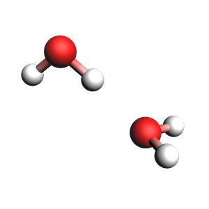
Create Dimer
Create an H2O dimer geometry and visualize it.
molecule = Molecule()

molecule.add_atom(Atom(symbol="O", coords=[0.000, 0.000, 0.000]))
molecule.add_atom(Atom(symbol="H", coords=[0.558, 0.598, -0.513]))
molecule.add_atom(Atom(symbol="H", coords=[0.028, -0.815, -0.512]))
molecule.add_atom(Atom(symbol="O", coords=[-0.066, 0.0230, 2.724]))
molecule.add_atom(Atom(symbol="H", coords=[0.000, 0.000, 1.749]))
molecule.add_atom(Atom(symbol="H", coords=[-0.956, 0.357, 2.838]))

view(molecule, width=300, height=300, guess_bonds=True, direction="tilt_y")
Run MD
Run NVT equilibration at 300 K with GFN1-xTB.
engine_settings = Settings()
engine_settings.input.DFTB.Model = "GFN1-xTB"

nvt_job = AMSNVTJob(
    molecule=molecule,
    settings=engine_settings,
    nsteps=20000,
    timestep=0.5,
    thermostat="Berendsen",
)
nvt_results = nvt_job.run();
[31.03|11:57:32] JOB plamsjob STARTED
[31.03|11:57:32] JOB plamsjob RUNNING
[31.03|11:59:56] JOB plamsjob FINISHED
[31.03|11:59:56] JOB plamsjob SUCCESSFUL
Restart from the equilibrated trajectory and run NVE production while logging dipole moments.
nve_job = AMSNVEJob.restart_from(nvt_job, binlog_dipolemoment=True)
nve_results = nve_job.run();
[31.03|11:59:56] JOB plamsjob STARTED
[31.03|11:59:56] Renaming job plamsjob to plamsjob.002
[31.03|11:59:56] JOB plamsjob.002 RUNNING
[31.03|12:02:03] JOB plamsjob.002 FINISHED
[31.03|12:02:03] JOB plamsjob.002 SUCCESSFUL
Set up autocorrelation analysis of dipole-moment derivatives to obtain the IR spectrum.
Run AMS Analysis
analysis_settings = Settings()
analysis_settings.input.TrajectoryInfo.Trajectory.KFFilename = nve_results.rkfpath()
analysis_settings.input.Task = "AutoCorrelation"
analysis_settings.input.AutoCorrelation.Property = "DipoleMomentFromBinLog"
analysis_settings.input.AutoCorrelation.UseTimeDerivative.Enabled = "Yes"
analysis_settings.input.AutoCorrelation.WritePropertyToKF = "Yes"
analysis_settings.input.AutoCorrelation.MaxCorrelationTime = 2000

analysis_job = AMSAnalysisJob(settings=analysis_settings)
analysis_results = analysis_job.run();
[31.03|12:13:07] JOB plamsjob STARTED
[31.03|12:13:07] Renaming job plamsjob to plamsjob.004
[31.03|12:13:07] JOB plamsjob.004 RUNNING
[31.03|12:13:08] JOB plamsjob.004 FINISHED
[31.03|12:13:08] JOB plamsjob.004 SUCCESSFUL
Extract Results
Write all generated analysis plots to text files and list the outputs.
plots = analysis_results.get_all_plots()
written_files = []
for plot in plots:
    filename = f"{plot.section}.txt"
    plot.write(filename)
    written_files.append(filename)

print("Wrote analysis files:")
for filename in written_files:
    print(f"- {filename}")
Wrote analysis files:
- AutoCorrelation_1.txt
- AutoCorrelationRaw_1.txt
- Spectrum_1.txt
- Integral_1.txt
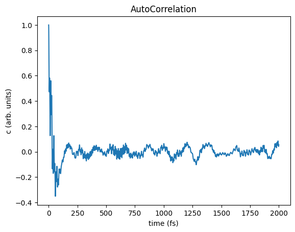
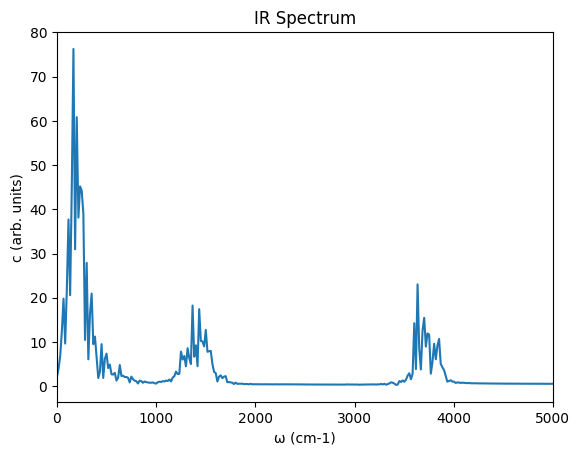
Finally, plot the autocorrelation function and IR spectrum.
ax = plots[0].plot(title="AutoCorrelation")
ax;
ax = plots[2].plot(xlim=(0, 5000), title="IR Spectrum")
ax;
See also
Python Script
#!/usr/bin/env python
# coding: utf-8

# ## IR Spectrum of H2O Dimer from MD
#
# Run an MD simulation with GFN1-xTB for a gas-phase water dimer, then compute the IR spectrum from dipole-moment autocorrelation with AMS trajectory analysis.
#

# This workflow can take some time to run, depending on hardware and MD length.
#

# ### Initial Imports

# Import PLAMS classes used for MD and analysis.
#

from pathlib import Path
from typing import List

from scm.plams import AMSAnalysisJob, AMSNVEJob, AMSNVTJob, Molecule, Atom, Settings, view


# ### Create Dimer

# Create an H2O dimer geometry and visualize it.
#

molecule = Molecule()

molecule.add_atom(Atom(symbol="O", coords=[0.000, 0.000, 0.000]))
molecule.add_atom(Atom(symbol="H", coords=[0.558, 0.598, -0.513]))
molecule.add_atom(Atom(symbol="H", coords=[0.028, -0.815, -0.512]))
molecule.add_atom(Atom(symbol="O", coords=[-0.066, 0.0230, 2.724]))
molecule.add_atom(Atom(symbol="H", coords=[0.000, 0.000, 1.749]))
molecule.add_atom(Atom(symbol="H", coords=[-0.956, 0.357, 2.838]))

view(molecule, width=300, height=300, guess_bonds=True, direction="tilt_y", picture_path="picture1.png")


# ### Run MD

# Run NVT equilibration at 300 K with GFN1-xTB.
#

engine_settings = Settings()
engine_settings.input.DFTB.Model = "GFN1-xTB"

nvt_job = AMSNVTJob(
    molecule=molecule,
    settings=engine_settings,
    nsteps=20000,
    timestep=0.5,
    thermostat="Berendsen",
)
nvt_results = nvt_job.run()
# Restart from the equilibrated trajectory and run NVE production while logging dipole moments.
#

nve_job = AMSNVEJob.restart_from(nvt_job, binlog_dipolemoment=True)
nve_results = nve_job.run()
# Set up autocorrelation analysis of dipole-moment derivatives to obtain the IR spectrum.
#

# ### Run AMS Analysis

analysis_settings = Settings()
analysis_settings.input.TrajectoryInfo.Trajectory.KFFilename = nve_results.rkfpath()
analysis_settings.input.Task = "AutoCorrelation"
analysis_settings.input.AutoCorrelation.Property = "DipoleMomentFromBinLog"
analysis_settings.input.AutoCorrelation.UseTimeDerivative.Enabled = "Yes"
analysis_settings.input.AutoCorrelation.WritePropertyToKF = "Yes"
analysis_settings.input.AutoCorrelation.MaxCorrelationTime = 2000

analysis_job = AMSAnalysisJob(settings=analysis_settings)
analysis_results = analysis_job.run()
# ### Extract Results

# Write all generated analysis plots to text files and list the outputs.
#

plots = analysis_results.get_all_plots()
written_files = []
for plot in plots:
    filename = f"{plot.section}.txt"
    plot.write(filename)
    written_files.append(filename)

print("Wrote analysis files:")
for filename in written_files:
    print(f"- {filename}")


# Finally, plot the autocorrelation function and IR spectrum.

ax = plots[0].plot(title="AutoCorrelation")
ax
ax.figure.savefig("picture2.png")


ax = plots[2].plot(xlim=(0, 5000), title="IR Spectrum")
ax
ax.figure.savefig("picture3.png")