PLUMED Biasing in AMS Molecular Dynamics¶

This example shows how to run AMS molecular dynamics with AMS restraints, the AMS EngineAddOn WallPotential, and PLUMED restraints.

In the demonstration, the reaction H2CO3(g) -> H2O(g) + CO2(g) is encouraged by a PLUMED MovingRestraint between one hydrogen and one oxygen atom, while the WallPotential keeps the product molecules close to each other.

Downloads: Notebook | Script ?

Requires: AMS2026 or later

../_images/ams_plumed_md_17_1_53c736c8.png

Initial imports¶

from scm.plams import *
from scm.base import ChemicalSystem, RKFTrajectory
import os
import numpy as np
import matplotlib.pyplot as plt

Initial system¶

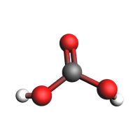
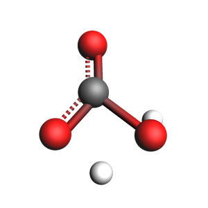
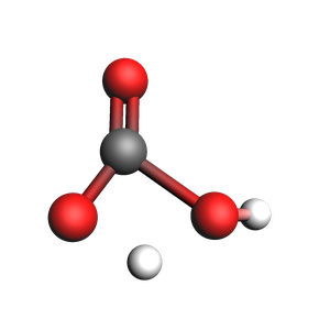
Define a Molecule from xyz coordinates and show the molecule.

O(3) is the right-most O atom
H(6) is the left-most H atom

mol = ChemicalSystem(
    """\
System
  Atoms
              O      -0.1009275285       1.5113007791      -0.4061554537
              C       0.0189044656       0.3835929386       0.1570043855
              O       1.2796450751      -0.2325516597       0.3936038789
              O      -1.0798994361      -0.4640886294       0.4005134306
              H       1.7530114719      -0.6822230417      -0.3461237499
              H      -1.8707340481      -0.5160303870      -0.1988424913
  End
End
"""
)

view(mol, guess_bonds=True, width=200, height=200)

Calculation settings¶

current_O3H6 = mol.get_distance(2, 5)
target_O3H6 = 0.95

print(
    f"Scanning bond O3-H6 from {current_O3H6:.3f} to {target_O3H6:.3f} angstrom (this will form a water molecule)"
)

current_O1C2 = mol.get_distance(0, 1)

print(f"Restraining bond O1-C2 at {current_O1C2:.3f} angstrom")

Scanning bond O3-H6 from 3.218 to 0.950 angstrom (this will form a water molecule)
Restraining bond O1-C2 at 1.266 angstrom

nsteps = 10000  # number of MD steps
kappa = 500000.0  # strength of Plumed MovingRestraint

s = Settings()
# run in serial
s.runscript.nproc = 1
s.runscript.preamble_lines = ["export OMP_NUM_THREADS=1"]

# engine settings
s.input.ReaxFF.ForceField = "CHO.ff"  # If you have ReaxFF license
# s.input.MLPotential.Model = 'M3GNet-UP-2022'   # if you have ML potential license and M3Gnet installed
# s.input.dftb  # if you have a DFTB license

# MD settings
s.input.ams.Task = "MolecularDynamics"
s.input.ams.MolecularDynamics.NSteps = nsteps
s.input.ams.MolecularDynamics.Trajectory.SamplingFreq = 100
s.input.ams.MolecularDynamics.InitialVelocities.Temperature = 200
s.input.ams.MolecularDynamics.Thermostat.Temperature = 500
s.input.ams.MolecularDynamics.Thermostat.Tau = 100
s.input.ams.MolecularDynamics.Thermostat.Type = "Berendsen"

# use an AMS restraint for one of the C-O bond lengths
s.input.ams.Restraints.Distance = []
s.input.ams.Restraints.Distance.append(f"1 2 {current_O1C2} 1.0")

# use an AMS EngineAddon WallPotential to keep the molecules within a sphere of radius 4 angstrom
s.input.ams.EngineAddons.WallPotential.Enabled = "Yes"
s.input.ams.EngineAddons.WallPotential.Radius = 4.0

# Plumed input, note that distances are given in nanometer so multiply by 0.1
s.input.ams.MolecularDynamics.Plumed.Input = f"""
    DISTANCE ATOMS=3,6 LABEL=d36
    MOVINGRESTRAINT ARG=d36 STEP0=1 AT0={current_O3H6 * 0.1} KAPPA0={kappa} STEP1={nsteps} AT1={target_O3H6 * 0.1}
    PRINT ARG=d36 FILE=colvar-d36.dat STRIDE=20
    End"""

job = AMSJob(settings=s, molecule=mol, name="dissociating-carbonic-acid")
print(job.get_input())

EngineAddons
  WallPotential
    Enabled Yes
    Radius 4.0
  End
End

MolecularDynamics
  InitialVelocities
    Temperature 200
... output trimmed ....
      H 1.7530114719 -0.6822230417 -0.3461237499
      H -1.8707340481 -0.516030387 -0.1988424913
   End
End

Engine ReaxFF
  ForceField CHO.ff
EndEngine

Run the job¶

job.run();

[08.04|17:36:24] JOB dissociating-carbonic-acid STARTED
[08.04|17:36:24] JOB dissociating-carbonic-acid RUNNING
[08.04|17:36:25] JOB dissociating-carbonic-acid FINISHED
[08.04|17:36:25] JOB dissociating-carbonic-acid SUCCESSFUL

Analyze the trajectory¶

Extract the O3H6 distances at each stored frame, and plot some of the molecules

trajectory = RKFTrajectory(job.results.rkfpath())

every = 20  # picture every 20 frames in the trajectory
O3H6_distances = []

imgs = {}
for i, it in enumerate(trajectory, 1):
    O3H6_distances.append(it.system.get_distance(2, 5))
    if i % every == 1:
        imgs[f"frame {it.frame_number}"] = view(it.system, width=200, height=200, guess_bonds=True)
plot_image_grid(imgs, rows=1);

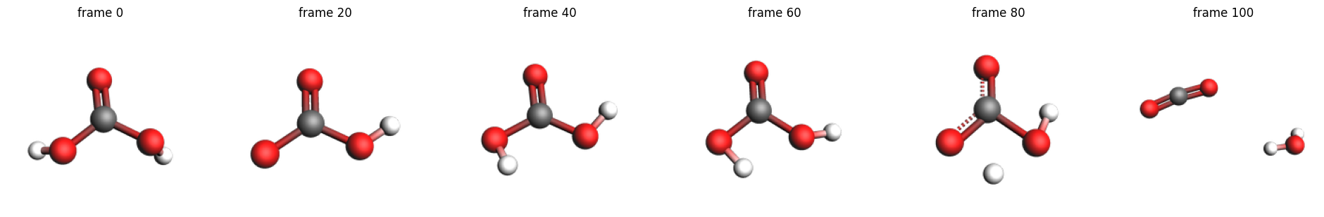
The above pictures show how the H(6) approaches the O(3). At the end, the carbonic acid molecule has dissociated into CO2 and H2O.

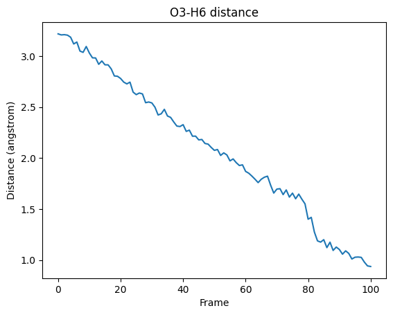
fig, ax = plt.subplots()
ax.plot(O3H6_distances)
ax.set_ylabel("Distance (angstrom)")
ax.set_xlabel("Frame")
ax.set_title("O3-H6 distance")
ax;

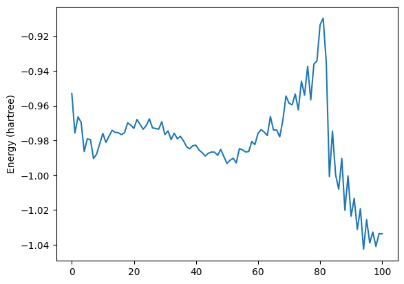
energies = job.results.get_history_property("Energy")
fig, ax = plt.subplots()
ax.plot(energies)
ax.set_ylabel("Energy (hartree)")
ax;

A transition state search¶

PLAMS makes it easy to extract any frame from an MD trajectory. As an example, let’s use highest-energy frame as an initial structure for a transition state search with the ADF DFT engine.

index = np.argmax(energies) + 1
approximate_ts_molecule = job.results.get_history_molecule(index)

print(f"Using frame {index} as initial approximate transition state:")
view(approximate_ts_molecule, width=300, height=300, guess_bonds=True)

Using frame 82 as initial approximate transition state:

ts_s = Settings()
ts_s.input.ams.task = "TransitionStateSearch"
ts_s.input.ams.GeometryOptimization.InitialHessian.Type = "Calculate"
ts_s.input.ams.Properties.NormalModes = "Yes"
ts_s.input.adf.xc.gga = "PBE"
ts_job = AMSJob(settings=ts_s, molecule=approximate_ts_molecule, name="ts-search")
ts_job.run();

[08.04|17:36:32] JOB ts-search STARTED
[08.04|17:36:32] JOB ts-search RUNNING
[08.04|17:36:59] JOB ts-search FINISHED
[08.04|17:36:59] JOB ts-search SUCCESSFUL

print("Optimized transition state:")
view(ts_job.results.get_main_system(), width=300, height=300, guess_bonds=True)

Optimized transition state:

print("Frequencies (at a TS there should be 1 imaginary [given as negative])")

for f in ts_job.results.get_frequencies():
    print(f"{f:.3f} cm^-1")

Frequencies (at a TS there should be 1 imaginary [given as negative])
-1434.162 cm^-1
754 cm^-1
582 cm^-1
310 cm^-1
049 cm^-1
927 cm^-1
041 cm^-1
855 cm^-1
610 cm^-1
164 cm^-1
177 cm^-1
995 cm^-1

Python Script¶

#!/usr/bin/env python
# coding: utf-8

# ## Initial imports

from scm.plams import *
from scm.base import ChemicalSystem, RKFTrajectory
import os
import numpy as np
import matplotlib.pyplot as plt


# ## Initial system
#
# Define a Molecule from xyz coordinates and show the molecule.
#
# * O(3) is the right-most O atom
# * H(6) is the left-most H atom

mol = ChemicalSystem(
    """\
System
  Atoms
              O      -0.1009275285       1.5113007791      -0.4061554537 
              C       0.0189044656       0.3835929386       0.1570043855
              O       1.2796450751      -0.2325516597       0.3936038789
              O      -1.0798994361      -0.4640886294       0.4005134306
              H       1.7530114719      -0.6822230417      -0.3461237499
              H      -1.8707340481      -0.5160303870      -0.1988424913
  End
End
"""
)

view(mol, guess_bonds=True, width=200, height=200, picture_path="picture1.png")


# ## Calculation settings

current_O3H6 = mol.get_distance(2, 5)
target_O3H6 = 0.95

print(f"Scanning bond O3-H6 from {current_O3H6:.3f} to {target_O3H6:.3f} angstrom (this will form a water molecule)")

current_O1C2 = mol.get_distance(0, 1)

print(f"Restraining bond O1-C2 at {current_O1C2:.3f} angstrom")


nsteps = 10000  # number of MD steps
kappa = 500000.0  # strength of Plumed MovingRestraint

s = Settings()
# run in serial
s.runscript.nproc = 1
s.runscript.preamble_lines = ["export OMP_NUM_THREADS=1"]

# engine settings
s.input.ReaxFF.ForceField = "CHO.ff"  # If you have ReaxFF license
# s.input.MLPotential.Model = 'M3GNet-UP-2022'   # if you have ML potential license and M3Gnet installed
# s.input.dftb  # if you have a DFTB license

# MD settings
s.input.ams.Task = "MolecularDynamics"
s.input.ams.MolecularDynamics.NSteps = nsteps
s.input.ams.MolecularDynamics.Trajectory.SamplingFreq = 100
s.input.ams.MolecularDynamics.InitialVelocities.Temperature = 200
s.input.ams.MolecularDynamics.Thermostat.Temperature = 500
s.input.ams.MolecularDynamics.Thermostat.Tau = 100
s.input.ams.MolecularDynamics.Thermostat.Type = "Berendsen"

# use an AMS restraint for one of the C-O bond lengths
s.input.ams.Restraints.Distance = []
s.input.ams.Restraints.Distance.append(f"1 2 {current_O1C2} 1.0")

# use an AMS EngineAddon WallPotential to keep the molecules within a sphere of radius 4 angstrom
s.input.ams.EngineAddons.WallPotential.Enabled = "Yes"
s.input.ams.EngineAddons.WallPotential.Radius = 4.0

# Plumed input, note that distances are given in nanometer so multiply by 0.1
s.input.ams.MolecularDynamics.Plumed.Input = f"""
    DISTANCE ATOMS=3,6 LABEL=d36
    MOVINGRESTRAINT ARG=d36 STEP0=1 AT0={current_O3H6 * 0.1} KAPPA0={kappa} STEP1={nsteps} AT1={target_O3H6 * 0.1}
    PRINT ARG=d36 FILE=colvar-d36.dat STRIDE=20
    End"""

job = AMSJob(settings=s, molecule=mol, name="dissociating-carbonic-acid")
print(job.get_input())


# ## Run the job

job.run()
# ## Analyze the trajectory
#
# Extract the O3H6 distances at each stored frame, and plot some of the molecules

trajectory = RKFTrajectory(job.results.rkfpath())

every = 20  # picture every 20 frames in the trajectory
O3H6_distances = []

imgs = {}
for i, it in enumerate(trajectory, 1):
    O3H6_distances.append(it.system.get_distance(2, 5))
    if i % every == 1:
        imgs[f"frame {it.frame_number}"] = view(it.system, width=200, height=200, guess_bonds=True)
plot_image_grid(imgs, rows=1, save_path="picture2.png")
# The above pictures show how the H(6) approaches the O(3). At the end, the carbonic acid molecule has dissociated into CO2 and H2O.

fig, ax = plt.subplots()
ax.plot(O3H6_distances)
ax.set_ylabel("Distance (angstrom)")
ax.set_xlabel("Frame")
ax.set_title("O3-H6 distance")
ax
ax.figure.savefig("picture3.png")


energies = job.results.get_history_property("Energy")
fig, ax = plt.subplots()
ax.plot(energies)
ax.set_ylabel("Energy (hartree)")
ax
ax.figure.savefig("picture4.png")


# ## A transition state search
#
# PLAMS makes it easy to extract any frame from an MD trajectory. As an example, let's use highest-energy frame as an initial structure for a transition state search with the ADF DFT engine.

index = np.argmax(energies) + 1
approximate_ts_molecule = job.results.get_history_molecule(index)

print(f"Using frame {index} as initial approximate transition state:")
view(approximate_ts_molecule, width=300, height=300, guess_bonds=True, picture_path="picture5.png")


ts_s = Settings()
ts_s.input.ams.task = "TransitionStateSearch"
ts_s.input.ams.GeometryOptimization.InitialHessian.Type = "Calculate"
ts_s.input.ams.Properties.NormalModes = "Yes"
ts_s.input.adf.xc.gga = "PBE"
ts_job = AMSJob(settings=ts_s, molecule=approximate_ts_molecule, name="ts-search")
ts_job.run()
print("Optimized transition state:")
view(ts_job.results.get_main_system(), width=300, height=300, guess_bonds=True, picture_path="picture6.png")


print("Frequencies (at a TS there should be 1 imaginary [given as negative])")

for f in ts_job.results.get_frequencies():
    print(f"{f:.3f} cm^-1")

PLUMED Biasing in AMS Molecular Dynamics¶

Initial imports¶

Initial system¶

Calculation settings¶

Run the job¶

Analyze the trajectory¶

A transition state search¶

See also¶

Related examples¶

Related tutorials¶

Related documentation¶

Python Script¶