ReaxFF Density Equilibration¶

Estimate the density predicted by ReaxFF for liquid water by starting from a low-density box, running a short NVT equilibration, scanning toward a target density with an MD deformation, and then continuing with an NPT simulation. The example shows how to inspect the density trace and extract a representative equilibrated structure.

Downloads: Notebook | Script ?

Requires: AMS2026 or later

ReaxFF density equilibration¶

Estimate the density predicted by ReaxFF for liquid water by starting from a low-density box, running a short NVT equilibration, using a deformation-based MD scan toward a target density, and then continuing with an NPT simulation. The example shows how to inspect the density trace and extract a representative equilibrated structure.

ReaxFF parallelizes with both MPI and OpenMP. To keep this example simple and reproducible, the run is configured in serial by setting nproc=1 and OMP_NUM_THREADS=1.

from scm.plams import Settings

reaxff_s = Settings()
reaxff_s.input.ReaxFF.ForceField = "Water2017.ff"
reaxff_s.runscript.nproc = 1
reaxff_s.runscript.preamble_lines = ["export OMP_NUM_THREADS=1"]

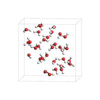
Start from a deliberately loose liquid box so the short NVT run can relax the molecular arrangement before the density scan and barostat are switched on.

from scm.plams import packmol, preoptimize, view, from_smiles

low_density_box = packmol(from_smiles("O"), n_molecules=32, region_names="water", density=0.4)
low_density_box = preoptimize(low_density_box, maxiterations=50)
view(low_density_box, height=200, width=200, direction="tilt_z")

Run a short NVT equilibration at the low starting density.

from scm.plams import AMSNVTJob

nvt_low_density_job = AMSNVTJob(
    molecule=low_density_box,
    name="nvt_low_density_job",
    settings=reaxff_s,
    nsteps=3000,
    temperature=300,
    thermostat="Berendsen",
    tau=100,
    samplingfreq=500,
    timestep=0.5,
)
nvt_low_density_job.run();

[23.03|16:47:51] JOB nvt_low_density_job STARTED
[23.03|16:47:51] JOB nvt_low_density_job RUNNING
[23.03|16:47:58] JOB nvt_low_density_job FINISHED
[23.03|16:47:58] JOB nvt_low_density_job SUCCESSFUL

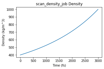
Use a regular AMSMDJob with a deformation toward a target density of 1.0 g/cm^3. This replaces the dedicated scan job while keeping the intermediate density-ramp stage explicit in the workflow.

from scm.plams import Settings, AMSMDJob

scan_density_settings = Settings()
scan_density_settings.input.ams.MolecularDynamics.Deformation.StartStep = 1
scan_density_settings.input.ams.MolecularDynamics.Deformation.StopStep = 6000
scan_density_settings.input.ams.MolecularDynamics.Deformation.TargetDensity = 1.0

scan_density_job = AMSMDJob.restart_from(
    nvt_low_density_job,
    name="scan_density_job",
    settings=reaxff_s,
    nsteps=6000,
    samplingfreq=100,
    temperature=300,
    thermostat="Berendsen",
    tau=100,
    timestep=0.5,
)
scan_density_job.settings += scan_density_settings
scan_density_job.run();

[23.03|16:47:58] JOB scan_density_job STARTED
[23.03|16:47:58] JOB scan_density_job RUNNING
[23.03|16:48:18] JOB scan_density_job FINISHED
[23.03|16:48:18] JOB scan_density_job SUCCESSFUL

import matplotlib.pyplot as plt
import numpy as np
from scm.base import Units


def plot_density(job, title=None, window: int = None):
    time = job.results.get_history_property("Time", "MDHistory")
    density = np.array(job.results.get_history_property("Density", "MDHistory"))
    density *= Units.conversion_factor("au", "kg") / Units.conversion_factor("bohr", "m") ** 3
    fig, ax = plt.subplots(figsize=(5, 3))
    ax.plot(time, density)
    ax.set_xlabel("Time (fs)")
    ax.set_ylabel("Density (kg/m^3)")
    ax.set_title(title or job.name + " Density")
    return ax


ax = plot_density(scan_density_job)
ax;

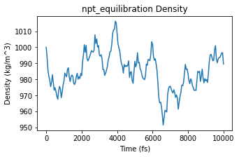
Continue with an NPT simulation from the final frame of the density-scan job.

from scm.plams import AMSNPTJob

npt_equilibration = AMSNPTJob.restart_from(
    scan_density_job,
    name="npt_equilibration",
    nsteps=20000,
    temperature=300,
    thermostat="Berendsen",
    tau=100,
    barostat="Berendsen",
    equal="XYZ",
    pressure=1e5,
    barostat_tau=1000,
)

npt_equilibration.run();

[23.03|16:56:16] JOB npt_equilibration STARTED
[23.03|16:56:16] JOB npt_equilibration RUNNING
[23.03|16:57:40] JOB npt_equilibration FINISHED
[23.03|16:57:40] JOB npt_equilibration SUCCESSFUL

ax = plot_density(npt_equilibration)
ax;

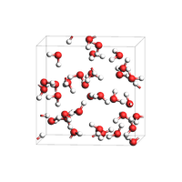
Extract a representative frame from the equilibrated part of the NPT trajectory. For production work, the simulation should generally be much longer before trusting the density.

from scm.plams import view

equilibrated_box = npt_equilibration.results.get_equilibrated_molecule()
print("Density: {:.2f} kg/m^3".format(equilibrated_box.get_density()))
equilibrated_box.write("water_equilibrated_box.xyz")
view(equilibrated_box, height=200, width=200, direction="tilt_z")

Density: 980.92 kg/m^3

Note: get_equilibrated_molecule() is only available for the AMSNPTJob class and by default gets a structure from the last third of the simulation with a density that is close to the average during that segment.

This is dfferent from get_main_molecule() which returns the final frame.

Python Script¶

#!/usr/bin/env python
# coding: utf-8

# ## ReaxFF density equilibration
#
# Estimate the density predicted by ReaxFF for liquid water by starting from a low-density box, running a short NVT equilibration, using a deformation-based MD scan toward a target density, and then continuing with an NPT simulation. The example shows how to inspect the density trace and extract a representative equilibrated structure.
#

# ReaxFF parallelizes with both MPI and OpenMP. To keep this example simple and reproducible, the run is configured in serial by setting ``nproc=1`` and ``OMP_NUM_THREADS=1``.
#

from scm.plams import Settings

reaxff_s = Settings()
reaxff_s.input.ReaxFF.ForceField = "Water2017.ff"
reaxff_s.runscript.nproc = 1
reaxff_s.runscript.preamble_lines = ["export OMP_NUM_THREADS=1"]


# Start from a deliberately loose liquid box so the short NVT run can relax the molecular arrangement before the density scan and barostat are switched on.
#

from scm.plams import packmol, preoptimize, view, from_smiles

low_density_box = packmol(from_smiles("O"), n_molecules=32, region_names="water", density=0.4)
low_density_box = preoptimize(low_density_box, maxiterations=50)
view(low_density_box, height=200, width=200, direction="tilt_z", picture_path="picture1.png")


# Run a short NVT equilibration at the low starting density.
#

from scm.plams import AMSNVTJob

nvt_low_density_job = AMSNVTJob(
    molecule=low_density_box,
    name="nvt_low_density_job",
    settings=reaxff_s,
    nsteps=3000,
    temperature=300,
    thermostat="Berendsen",
    tau=100,
    samplingfreq=500,
    timestep=0.5,
)
nvt_low_density_job.run()
# Use a regular ``AMSMDJob`` with a deformation toward a target density of ``1.0 g/cm^3``. This replaces the dedicated scan job while keeping the intermediate density-ramp stage explicit in the workflow.
#

from scm.plams import Settings, AMSMDJob

scan_density_settings = Settings()
scan_density_settings.input.ams.MolecularDynamics.Deformation.StartStep = 1
scan_density_settings.input.ams.MolecularDynamics.Deformation.StopStep = 6000
scan_density_settings.input.ams.MolecularDynamics.Deformation.TargetDensity = 1.0

scan_density_job = AMSMDJob.restart_from(
    nvt_low_density_job,
    name="scan_density_job",
    settings=reaxff_s,
    nsteps=6000,
    samplingfreq=100,
    temperature=300,
    thermostat="Berendsen",
    tau=100,
    timestep=0.5,
)
scan_density_job.settings += scan_density_settings
scan_density_job.run()
import matplotlib.pyplot as plt
import numpy as np
from scm.base import Units


def plot_density(job, title=None, window: int = None):
    time = job.results.get_history_property("Time", "MDHistory")
    density = np.array(job.results.get_history_property("Density", "MDHistory"))
    density *= Units.conversion_factor("au", "kg") / Units.conversion_factor("bohr", "m") ** 3
    fig, ax = plt.subplots(figsize=(5, 3))
    ax.plot(time, density)
    ax.set_xlabel("Time (fs)")
    ax.set_ylabel("Density (kg/m^3)")
    ax.set_title(title or job.name + " Density")
    return ax


ax = plot_density(scan_density_job)
ax
ax.figure.savefig("picture2.png")


# Continue with an NPT simulation from the final frame of the density-scan job.
#

from scm.plams import AMSNPTJob

npt_equilibration = AMSNPTJob.restart_from(
    scan_density_job,
    name="npt_equilibration",
    nsteps=20000,
    temperature=300,
    thermostat="Berendsen",
    tau=100,
    barostat="Berendsen",
    equal="XYZ",
    pressure=1e5,
    barostat_tau=1000,
)

npt_equilibration.run()
ax = plot_density(npt_equilibration)
ax
ax.figure.savefig("picture3.png")


# Extract a representative frame from the equilibrated part of the NPT trajectory. For production work, the simulation should generally be much longer before trusting the density.
#

from scm.plams import view

equilibrated_box = npt_equilibration.results.get_equilibrated_molecule()
print("Density: {:.2f} kg/m^3".format(equilibrated_box.get_density()))
equilibrated_box.write("water_equilibrated_box.xyz")
view(equilibrated_box, height=200, width=200, direction="tilt_z", picture_path="picture4.png")


# Note: `get_equilibrated_molecule()` is only available for the AMSNPTJob class and by default gets a structure from the last third of the simulation with a density that is close to the average during that segment.
#
# This is dfferent from `get_main_molecule()` which returns the final frame.

ReaxFF Density Equilibration¶

ReaxFF density equilibration¶

See also¶

Related examples¶

Related tutorials¶

Related documentation¶

Python Script¶