Diffusion Coefficient Supercell Dependence
Run Lennard-Jones argon simulations for several box sizes, calculate diffusion coefficients from the mean-squared displacement, and extrapolate the results to infinite system size with a linear fit in 1/L.
Diffusion coefficient supercell dependence
Finite-size effects make the diffusion coefficient depend on the size of the simulation cell. This example runs Lennard-Jones argon boxes of different sizes, computes the diffusion coefficient from the mean-squared displacement, and linearly extrapolates the results to the infinite-system limit.
from scm.plams import Settings


def get_lennard_jones_settings():
    s = Settings()
    s.input.lennardjones.eps = 3.785e-4
    s.input.lennardjones.rmin = 3.81637
    s.input.lennardjones.cutoff = 8.0
    s.runscript.nproc = 1
    return s
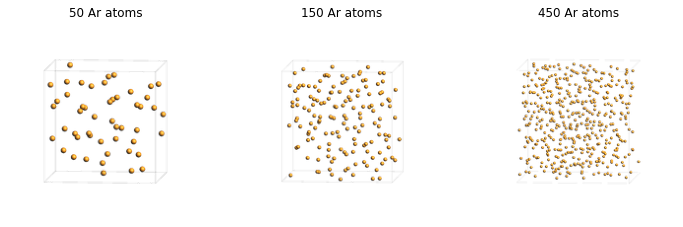
Set up three argon boxes at the same density and visualize the resulting supercells.
from scm.plams import Molecule, Atom, packmol, preoptimize, plot_image_grid, view

sizes = [50, 150, 450]
inverted_L_list = []
density = 1.0  # g/cm^3

Ar = Molecule()
Ar.add_atom(Atom(symbol="Ar", coords=(0, 0, 0)))

boxes = []
imgs = {}
for size in sizes:
    mol = packmol(Ar, n_molecules=size, density=density)
    mol = preoptimize(mol, settings=get_lennard_jones_settings(), maxiterations=50)
    boxes.append(mol)
    L = mol.lattice[0][0]
    inverted_L_list.append(1.0 / L)
    print(f"{size} Ar atoms, density = {density} g/cm^3")
    imgs[f"{size} Ar atoms"] = view(mol, height=200, width=200, direction="tilt_z")

plot_image_grid(imgs, rows=1);
50 Ar atoms, density = 1.0 g/cm^3
150 Ar atoms, density = 1.0 g/cm^3
450 Ar atoms, density = 1.0 g/cm^3
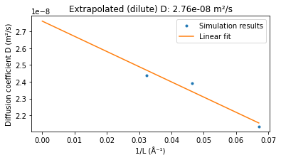
For each system, run an NVT equilibration, an NVT production simulation, and an MSD analysis. The diffusion coefficients are then fitted as a function of 1/L.
D_list = []
temperature = 400
max_correlation_time_fs = 6000
start_time_fit_fs = 3000
from scm.plams import AMSNVTJob, AMSMSDJob, log

for size, mol in zip(sizes, boxes):
    eq_job = AMSNVTJob(
        name=f"eq_{size}",
        settings=get_lennard_jones_settings(),
        molecule=mol,
        temperature=temperature,
        nsteps=10000,
        samplingfreq=500,
        thermostat="Berendsen",
        tau=100,
        timestep=1.0,
        writebonds=False,
        writecharges=False,
        writemolecules=False,
        writevelocities=False,
    )
    eq_job.run()
    prod_job = AMSNVTJob.restart_from(
        eq_job,
        name=f"prod_{size}",
        nsteps=60000,
        samplingfreq=25,
        temperature=temperature,
        thermostat="NHC",
    )
    prod_job.run()
    msd_job = AMSMSDJob(
        prod_job, name=f"msd_{size}", max_correlation_time_fs=max_correlation_time_fs
    )
    msd_job.run()
    D = msd_job.results.get_diffusion_coefficient(start_time_fit_fs=start_time_fit_fs)
    D_list.append(D)
    log(f"{size} atoms: D = {D:.2e} m^2 s^-1")
[23.03|16:01:20] JOB eq_50 STARTED
[23.03|16:01:20] JOB eq_50 RUNNING
[23.03|16:01:22] JOB eq_50 FINISHED
[23.03|16:01:22] JOB eq_50 SUCCESSFUL
[23.03|16:01:22] JOB prod_50 STARTED
[23.03|16:01:22] JOB prod_50 RUNNING
[23.03|16:01:34] JOB prod_50 FINISHED
[23.03|16:01:34] JOB prod_50 SUCCESSFUL
[23.03|16:01:34] JOB msd_50 STARTED
[23.03|16:01:34] JOB msd_50 RUNNING
... output trimmed ....
[23.03|16:02:21] JOB eq_450 SUCCESSFUL
[23.03|16:02:21] JOB prod_450 STARTED
[23.03|16:02:21] JOB prod_450 RUNNING
[23.03|16:03:40] JOB prod_450 FINISHED
[23.03|16:03:41] JOB prod_450 SUCCESSFUL
[23.03|16:03:41] JOB msd_450 STARTED
[23.03|16:03:41] JOB msd_450 RUNNING
[23.03|16:03:42] JOB msd_450 FINISHED
[23.03|16:03:42] JOB msd_450 SUCCESSFUL
[23.03|16:03:42] 450 atoms: D = 2.44e-08 m^2 s^-1
import matplotlib.pyplot as plt
from scm.plams import log
from scm.plams.tools.plot import linear_fit_extrapolate_to_0

fit_x, fit_y, slope, intercept = linear_fit_extrapolate_to_0(inverted_L_list, D_list)

dilute_D = intercept
title = f"Extrapolated (dilute) D: {dilute_D:.2e} m²/s"
log(title)

fig, ax = plt.subplots(figsize=(6, 3))
ax.plot(inverted_L_list, D_list, ".", label="Simulation results")
ax.plot(fit_x, fit_y, label="Linear fit")
ax.set_title(title)
ax.legend()
ax.set_xlabel("1/L (Å⁻¹)")
ax.set_ylabel("Diffusion coefficient D (m²/s)")
ax;
[23.03|16:03:42] Extrapolated (dilute) D: 2.76e-08 m²/s
See also
Python Script
#!/usr/bin/env python
# coding: utf-8

# ## Diffusion coefficient supercell dependence
#
# Finite-size effects make the diffusion coefficient depend on the size of the simulation cell. This example runs Lennard-Jones argon boxes of different sizes, computes the diffusion coefficient from the mean-squared displacement, and linearly extrapolates the results to the infinite-system limit.
#

from scm.plams import Settings


def get_lennard_jones_settings():
    s = Settings()
    s.input.lennardjones.eps = 3.785e-4
    s.input.lennardjones.rmin = 3.81637
    s.input.lennardjones.cutoff = 8.0
    s.runscript.nproc = 1
    return s


# Set up three argon boxes at the same density and visualize the resulting supercells.

from scm.plams import Molecule, Atom, packmol, preoptimize, plot_image_grid, view

sizes = [50, 150, 450]
inverted_L_list = []
density = 1.0  # g/cm^3

Ar = Molecule()
Ar.add_atom(Atom(symbol="Ar", coords=(0, 0, 0)))

boxes = []
imgs = {}
for size in sizes:
    mol = packmol(Ar, n_molecules=size, density=density)
    mol = preoptimize(mol, settings=get_lennard_jones_settings(), maxiterations=50)
    boxes.append(mol)
    L = mol.lattice[0][0]
    inverted_L_list.append(1.0 / L)
    print(f"{size} Ar atoms, density = {density} g/cm^3")
    imgs[f"{size} Ar atoms"] = view(mol, height=200, width=200, direction="tilt_z")

plot_image_grid(imgs, rows=1)
# For each system, run an NVT equilibration, an NVT production simulation, and an MSD analysis. The diffusion coefficients are then fitted as a function of ``1/L``.
#

D_list = []
temperature = 400
max_correlation_time_fs = 6000
start_time_fit_fs = 3000


from scm.plams import AMSNVTJob, AMSMSDJob, log

for size, mol in zip(sizes, boxes):
    eq_job = AMSNVTJob(
        name=f"eq_{size}",
        settings=get_lennard_jones_settings(),
        molecule=mol,
        temperature=temperature,
        nsteps=10000,
        samplingfreq=500,
        thermostat="Berendsen",
        tau=100,
        timestep=1.0,
        writebonds=False,
        writecharges=False,
        writemolecules=False,
        writevelocities=False,
    )
    eq_job.run()
    prod_job = AMSNVTJob.restart_from(
        eq_job,
        name=f"prod_{size}",
        nsteps=60000,
        samplingfreq=25,
        temperature=temperature,
        thermostat="NHC",
    )
    prod_job.run()
    msd_job = AMSMSDJob(prod_job, name=f"msd_{size}", max_correlation_time_fs=max_correlation_time_fs)
    msd_job.run()
    D = msd_job.results.get_diffusion_coefficient(start_time_fit_fs=start_time_fit_fs)
    D_list.append(D)
    log(f"{size} atoms: D = {D:.2e} m^2 s^-1")


import matplotlib.pyplot as plt
from scm.plams import log
from scm.plams.tools.plot import linear_fit_extrapolate_to_0

fit_x, fit_y, slope, intercept = linear_fit_extrapolate_to_0(inverted_L_list, D_list)

dilute_D = intercept
title = f"Extrapolated (dilute) D: {dilute_D:.2e} m²/s"
log(title)

fig, ax = plt.subplots(figsize=(6, 3))
ax.plot(inverted_L_list, D_list, ".", label="Simulation results")
ax.plot(fit_x, fit_y, label="Linear fit")
ax.set_title(title)
ax.legend()
ax.set_xlabel("1/L (Å⁻¹)")
ax.set_ylabel("Diffusion coefficient D (m²/s)")
ax
ax.figure.savefig("picture1.png")