Building Surfaces and Slabs
Create slabs from bulk ChemicalSystem objects with make_slab_layers() and make_slab_thickness(). The example also illustrates helpful use cases for make_supercell(), make_supercell_trafo(), guess_bonds(), map_atoms(), and map_atoms_continuous().
Building slabs from bulk ChemicalSystem objects
Miller indices identify crystal planes. For most cells, use the three-index notation (h, k, l).
Hexagonal cells are often written with four indices (h, k, i, l), where i = -(h + k).
We can call
cs.make_slab_layers((h, k, l), 6)# 6 layerscs.make_slab_layers((h, k, i, l), 6)# 6 layers, hexagonal cellcs.make_slab_thickness((h, k, l), -10.0, 0.0)# keep atoms between z=-10 and z=0
Note 1: make_slab_layers will return a slab with the same stoichiometry as the bulk material. make_slab_thickness may give you a different stoichoimetry, since it just cuts at certain z coordinates. So only use make_slab_thickness if the stoichiometry is not crucial (e.g. for a metal slab).
Note 2: Always start from the conventional unit cell before making a slab. This is because the Miller indices (by convention) refer to planes derived from the conventional cell.
from scm.base import ChemicalSystem
from scm.plams import view
fcc Cu(001)
copper_bulk = ChemicalSystem("""
System
    Atoms
        Cu 0.0 0.0 0.0
        Cu 0.0 1.805 1.805
        Cu 1.805 0.0 1.805
        Cu 1.805 1.805 0.0
    End
    Lattice
        3.61 0.0 0.0
        0.0 3.61 0.0
        0.0 0.0 3.61
    End
End
""")
view(copper_bulk, guess_bonds=True, direction="tilt_z")
Create the slab and show it tilted on its side (“tilt_x”):
slab = copper_bulk.make_slab_layers((0, 0, 1), 4)
view(slab, guess_bonds=True, direction="tilt_x")
fcc Cu(110)
slab = copper_bulk.make_slab_layers((1, 1, 0), 4)
view(slab, guess_bonds=True, direction="tilt_x")
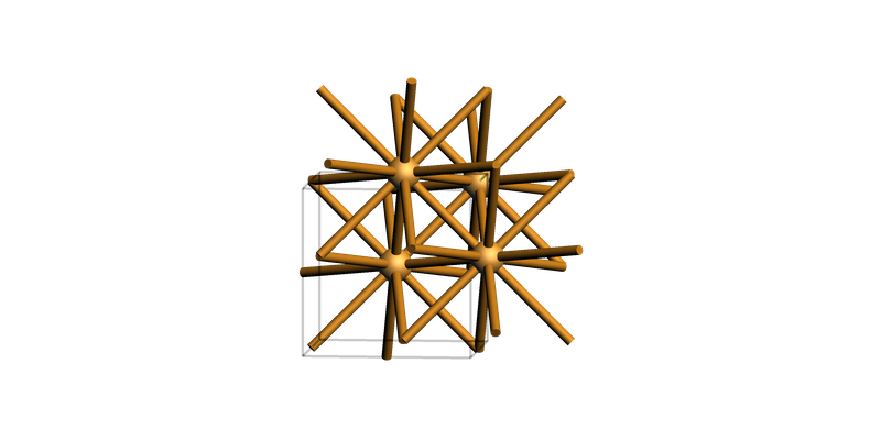
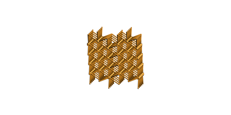
fcc Cu(111) hexagonal supercell
slab = copper_bulk.make_slab_layers((1, 1, 1), 6)
view(slab, guess_bonds=True, direction="tilt_x")
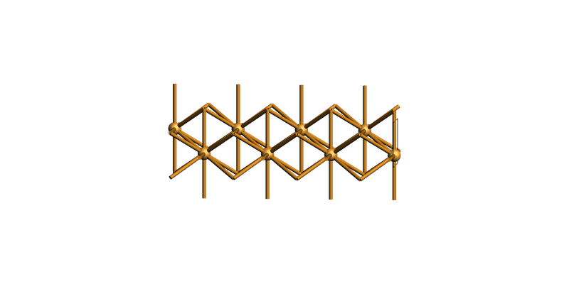
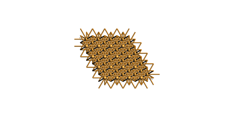
You can also create a supercell (side view):
slab_supercell = slab.make_supercell((4, 4))
view(slab_supercell, guess_bonds=True, direction="tilt_x")
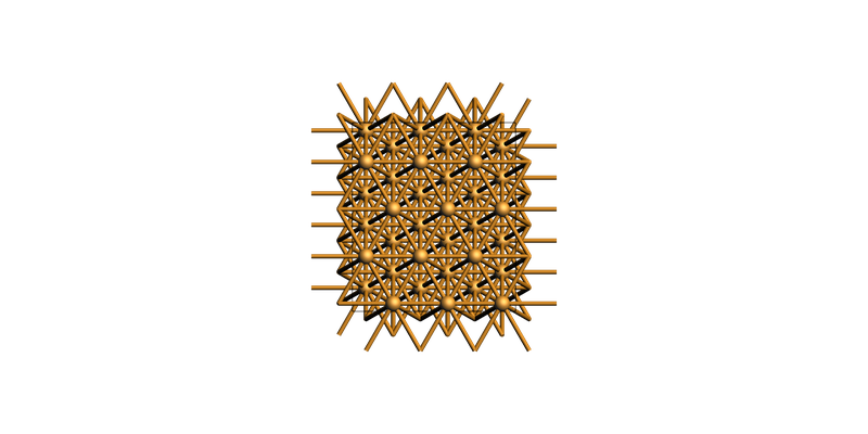
Or view it from a top view:
print(slab_supercell.lattice)
view(slab_supercell, guess_bonds=True, direction="along_z")
Lattice
   10.210621920333745 0 0
   -5.105310960166868 8.842657971447268 0
End
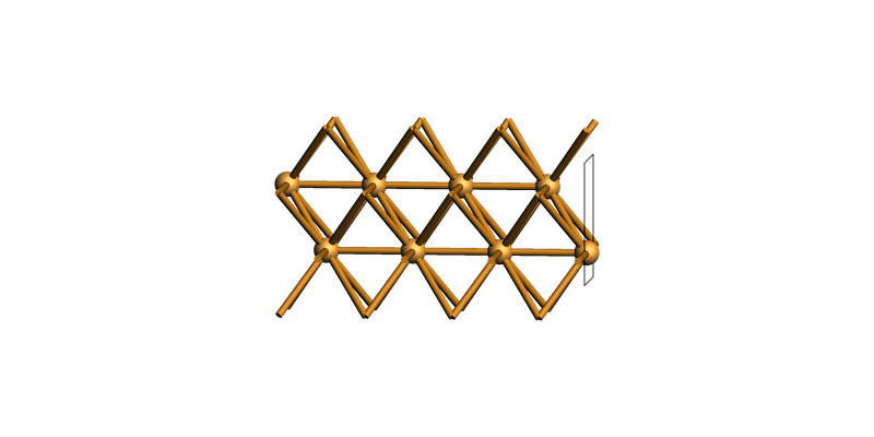
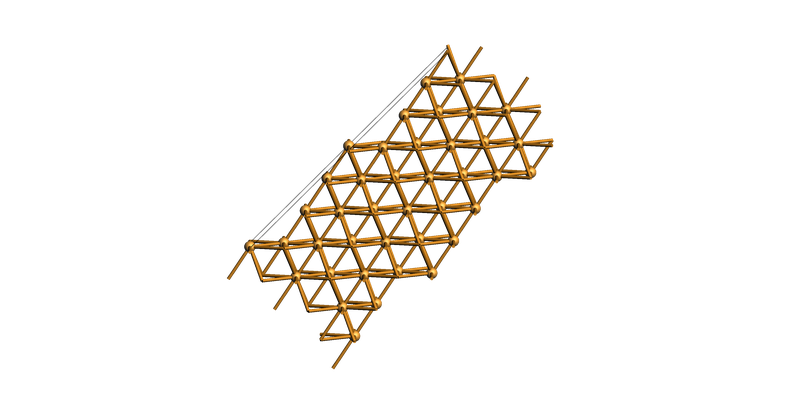
fcc Cu(111) rectangular supercell
slab = copper_bulk.make_slab_layers((1, 1, 1), 6)
slab_supercell = slab.make_supercell_trafo([[1, 0], [1, 2]])  # smallest rectangular supercell
slab_supercell.map_atoms(0.0)
print(slab_supercell.lattice)
view(slab_supercell, guess_bonds=True, direction="along_z")
Lattice
   2.5526554800834362 0 0
   1.8800151156845855e-15 4.421328985723634 0
End

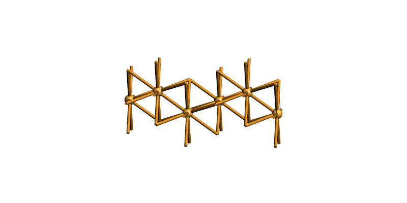
Or create a bigger rectangular supercell:
slab_supercell = slab.make_supercell_trafo([[3, 0], [2, 4]])
slab_supercell.map_atoms(0.0)
print(slab_supercell.lattice)
view(slab_supercell, guess_bonds=True, direction="along_z")
Lattice
   7.657966440250308 0 0
   3.760030231369171e-15 8.842657971447268 0
End
Build the vicinal stepped Cu(711) surface
slab = copper_bulk.make_slab_layers((7, 1, 1), 20)
view(slab, guess_bonds=True, direction="tilt_y")
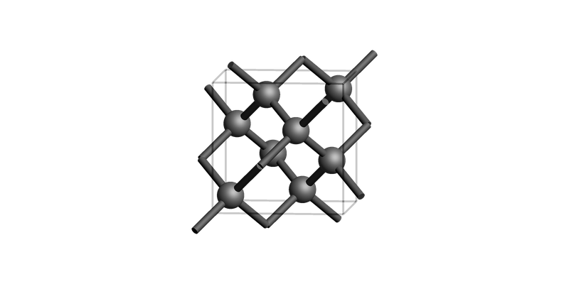
Diamond bulk conventional unit cell
diamond_bulk = ChemicalSystem(
    """\
System
   Atoms
       C 3.12375 3.12375 3.12375
       C 0.4462500000000001 0.4462500000000001 0.4462500000000001
       C 3.12375 1.33875 1.33875
       C 0.4462500000000001 2.23125 2.23125
       C 1.33875 3.12375 1.33875
       C 2.23125 0.4462500000000001 2.23125
       C 1.33875 1.33875 3.12375
       C 2.23125 2.23125 0.4462500000000001
   End
   Lattice
       3.57 0.0 0.0
       0.0 3.57 0.0
       0.0 0.0 3.57
   End
End"""
)

print("Diamond bulk")
view(diamond_bulk, guess_bonds=True, direction="tilt_x")
Diamond bulk
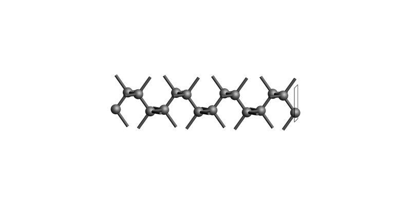
Diamond(001): make_slab_layers()
The slab is shown tilted on its side, so the top-most surface (with the rectangle outline) shows the surface.
diamond_layers_case_1 = diamond_bulk.make_slab_layers([0, 0, 1], 4)
print("Diamond slab: make_slab_layers([0, 0, 1], 2)")
view(diamond_layers_case_1, guess_bonds=True, direction="tilt_x")
Diamond slab: make_slab_layers([0, 0, 1], 2)
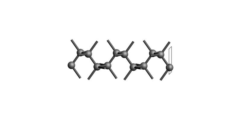
Diamond(001): make_slab_thickness()
Cut the slab between z-coordinates -10.0 and 0.0:
diamond_thickness_case_5 = diamond_bulk.make_slab_thickness([0, 0, 1], 0.0, -10.0, 0.0)
print("Diamond slab: make_slab_thickness([0, 0, 1], 0.0, -10.0, 0.0)")
view(diamond_thickness_case_5, guess_bonds=True, direction="tilt_x")
Diamond slab: make_slab_thickness([0, 0, 1], 0.0, -10.0, 0.0)
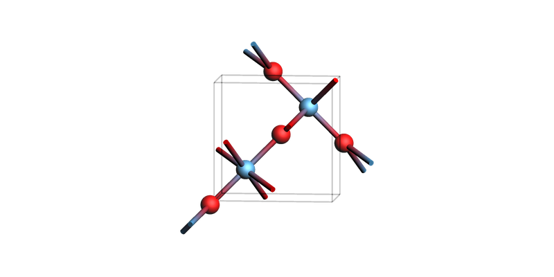
Hexagonal ZnO(10-10): three-index and four-index Miller notation
zno_bulk = ChemicalSystem(
    """\
System
    Atoms
        Zn -2.220446049250313e-16 1.876388373333333 0.0
        Zn 1.625 0.9381941866666664 2.615
        O -2.220446049250313e-16 1.876388373333333 1.961249999999999
        O 1.625 0.9381941866666664 4.576249999999999
    End
    Lattice
        3.25 0.0 0.0
        -1.625 2.81458256 0.0
        0.0 0.0 5.23
    End
End
"""
)

print("Wurtzite ZnO bulk")
view(zno_bulk, guess_bonds=True, direction="tilt_x")
Wurtzite ZnO bulk
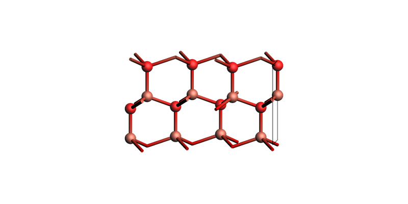
zno_layers_3index = zno_bulk.make_slab_layers([1, 0, 0], 4)
print("ZnO slab: make_slab_layers([1, 0, 0], 4)")
view(zno_layers_3index, guess_bonds=True, direction="tilt_x")
ZnO slab: make_slab_layers([1, 0, 0], 4)

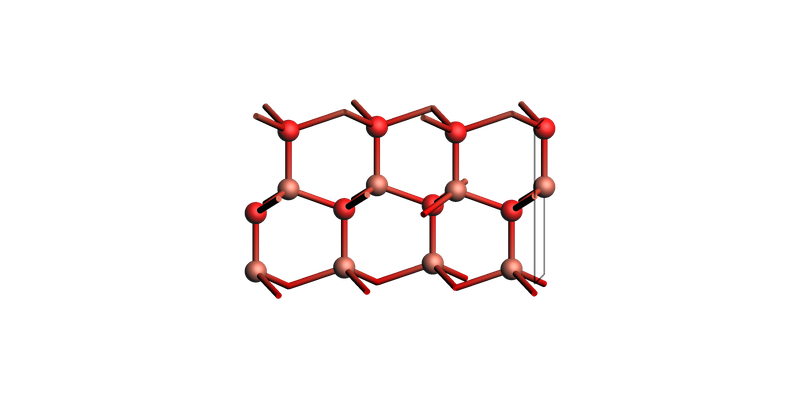
The corresponding 4-Miller-index notation:
zno_layers_4index = zno_bulk.make_slab_layers([1, 0, -1, 0], 4)
view(zno_layers_4index, guess_bonds=True, direction="tilt_x")
ZnO slab: make_slab_layers([1, 0, -1, 0], 4)
The three first indices in four-index Miller notation can be switched around:
zno_layers_4index = zno_bulk.make_slab_layers([1, -1, 0, 0], 4)
view(zno_layers_4index, guess_bonds=True, direction="tilt_x")
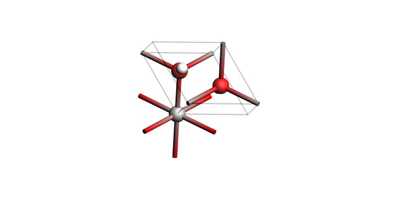
Brucite Mg(OH)2 (0001)
Brucite bulk
brucite_bulk = ChemicalSystem(
    """
    System
        Atoms
            Mg 0.0 0.0 0.0
            O 0.0 1.8140345458 1.0561456
            O 1.571 0.9070172729 3.7098544
            H 0.0 1.8140345458 2.0508098
            H 1.571 0.9070172729 2.7151902
        End
        Lattice
            3.142 0.0 0.0
            -1.571 2.7210518187 0.0
            0.0 0.0 4.766
        End
    End
    """
)
view(brucite_bulk, guess_bonds=True, direction="tilt_z")
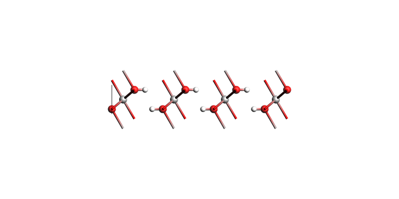
Brucite Mg(OH)2 (0001) make_slab_layers
slab = brucite_bulk.make_slab_layers((0, 0, 0, 1), 6)
view(slab, guess_bonds=True, direction="along_x")
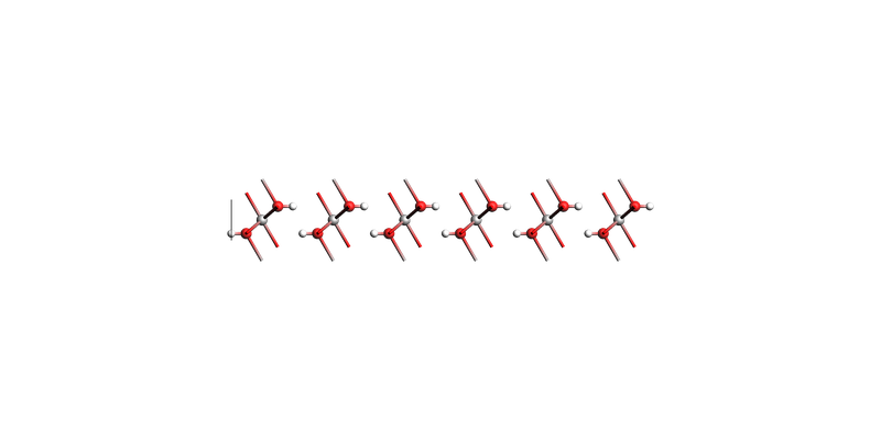
Brucite Mg(OH)2 (0001) make_slab_thickness
Note: some hydrogens get cut off in this example! This may not be what you want. make_slab_thickness does not preserve stoichoimetry.
slab = brucite_bulk.make_slab_thickness((0, 0, 0, 1), 0.0, -17.0)
view(slab, guess_bonds=True, direction="along_x")
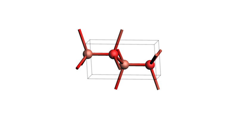
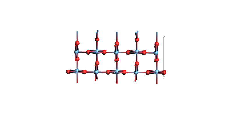
Rutile TiO2(110)
tio2_bulk = ChemicalSystem(
    """\
System
    Atoms
        Ti 0.0 0.0 0.0
        Ti 2.295 2.295 1.48
        O 3.672 0.918 1.48
        O 0.918 3.672 1.48
        O 1.377 1.377 0.0
        O -1.377 -1.377 0.0
    End
    Lattice
        4.59 0.0 0.0
        0.0 4.59 0.0
        0.0 0.0 2.96
    End
End"""
)

print("Titania bulk")
view(tio2_bulk, guess_bonds=True, direction="tilt_z")
Titania bulk
tio2_slab = tio2_bulk.make_slab_layers([1, 1, 0], 5)
print("Titania slab: make_slab_layers([1, 1, 0], 5)")
view(tio2_slab, guess_bonds=True, direction="tilt_x")
Titania slab: make_slab_layers([1, 1, 0], 5)
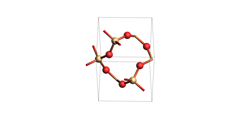
SiO2
sio2_bulk = ChemicalSystem(
    """\
System
    Atoms
        Si 1.15385 -1.998526824313349 3.606666666666666
        Si 1.15385 1.998526824313349 1.803333333333333
        Si 2.6023 0.0 0.0
        O 1.720955 -0.5485318305030256 4.25767
        O 2.069565 -2.487528068560232 2.454336666666666
        O 3.57448 -1.216124833518336 0.6510033333333325
        O 1.720955 0.5485318305030256 1.152330000000001
        O 2.069565 2.487528068560232 2.955663333333333
        O 3.57448 1.216124833518336 4.758996666666667
    End
    Lattice
        2.455 -4.252184732581593 0.0
        2.455 4.252184732581593 0.0
        0.0 0.0 5.41
    End
End"""
)

print("SiO2 bulk")
view(sio2_bulk, guess_bonds=True, direction="tilt_x")
SiO2 bulk
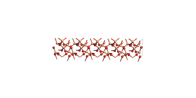
sio2_slab = sio2_bulk.make_slab_layers([0, 0, 1], 5)
print("SiO2 slab: make_slab_layers([0, 0, 1], 5)")
view(sio2_slab, guess_bonds=True, direction="tilt_x")
SiO2 slab: make_slab_layers([0, 0, 1], 5)
Naphthalene
For molecular crystals like naphthalene, it may be difficult to cut slabs without cutting through the molecules. Always carefully check the resulting slab before using it in a calculation!
naphthalene_bulk = ChemicalSystem(
"""\
System
Atoms
C -0.87388368 0.11073012 2.36589887
C 0.15273024 3.05568012 4.76889870
C 4.17013024 5.77916988 4.76889870
C 3.14351632 2.83421988 2.36589887
H -1.09410897 0.35103804 3.23705766
H 0.37295554 3.29598804 3.89773991
H 4.39035554 5.53886196 3.89773991
H 2.92329103 2.59391196 3.23705766
C -0.12579372 0.96653259 1.59034638
C -0.59535971 3.91148259 5.54445119
C 3.42204029 4.92336741 5.54445119
C 3.89160628 1.97841741 1.59034638
H 0.15997330 1.77874980 1.94280538
H -0.88112673 4.72369980 5.19199219
H 3.13627327 4.11115020 5.19199219
H 4.17737330 1.16620020 1.94280538
C 0.21357858 0.61726152 0.25185835
C -0.93473202 3.56221152 6.88293921
C 3.08266798 5.27263848 6.88293921
C 4.23097858 2.32768848 0.25185835
C -3.75675609 1.48307682 6.55901941
C 3.03560266 4.42802682 0.57577816
C 7.05300266 4.40682318 0.57577816
C 0.26064391 1.46187318 6.55901941
H -3.47488266 2.30353989 6.89435489
H 2.75372923 5.24848989 0.24044268
H 6.77112923 3.58636011 0.24044268
H 0.54251734 0.64141011 6.89435489
C 6.72508585 4.75845021 1.84862605
C 0.58856072 1.81350021 5.28617152
C -3.42883928 1.13144979 5.28617152
C 2.70768585 4.07639979 1.84862605
H 6.21662119 4.18477395 2.37588759
H 1.09702538 1.23982395 4.75890998
H -2.92037462 1.70512605 4.75890998
H 2.19922119 4.65007605 2.37588759
End
Lattice
8.03480000 0.00000000 0.00000000
0.00000000 5.88990000 0.00000000
-4.73855343 0.00000000 7.13479757
End
End"""
)
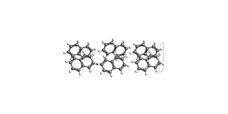
print("Naphthalene bulk")
view(naphthalene_bulk, guess_bonds=True, direction="tilt_z")
Naphthalene bulk
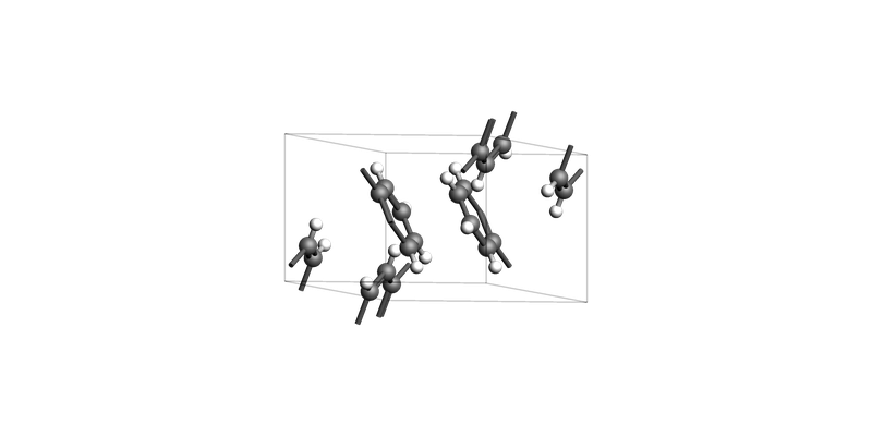
After making the slab, we call guess_bonds() and map_atoms_continuous() to make the visualization nicer:
naphthalene_slab_001 = naphthalene_bulk.make_slab_layers([0, 0, 1], 3)
naphthalene_slab_001.guess_bonds()
naphthalene_slab_001.map_atoms_continuous()
print("Naphthalene slab: make_slab_layers([0, 0, 1], 3)")
view(naphthalene_slab_001, guess_bonds=True, direction="tilt_x")
Naphthalene slab: make_slab_layers([0, 0, 1], 3)
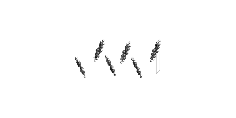
naphthalene_slab_100 = naphthalene_bulk.make_slab_layers([1, 0, 0], 3)
naphthalene_slab_100.guess_bonds()
naphthalene_slab_100.map_atoms_continuous()
print("Naphthalene slab: make_slab_layers([1, 0, 0], 3)")
view(naphthalene_slab_100, guess_bonds=True, direction="tilt_x")
Naphthalene slab: make_slab_layers([1, 0, 0], 3)
See also
Python Script
#!/usr/bin/env python
# coding: utf-8

# ## Building slabs from bulk `ChemicalSystem` objects
#
# Miller indices identify crystal planes. For most cells, use the three-index notation `(h, k, l)`.
#
# Hexagonal cells are often written with four indices `(h, k, i, l)`, where `i = -(h + k)`.
#
# We can call
#
# * `cs.make_slab_layers((h, k, l), 6)`  # 6 layers
# * `cs.make_slab_layers((h, k, i, l), 6)`  # 6 layers, hexagonal cell
# * `cs.make_slab_thickness((h, k, l), -10.0, 0.0)`  # keep atoms between z=-10 and z=0
#
# Note 1: `make_slab_layers` will return a slab with the same stoichiometry as the bulk material. `make_slab_thickness` may give you a different stoichoimetry, since it just cuts at certain z coordinates. So only use `make_slab_thickness` if the stoichiometry is not crucial (e.g. for a metal slab).
#
# Note 2: Always start from the conventional unit cell before making a slab. This is because the Miller indices (by convention) refer to planes derived from the conventional cell.

from scm.base import ChemicalSystem
from scm.plams import view


# ## fcc Cu(001)

copper_bulk = ChemicalSystem("""
System
    Atoms
        Cu 0.0 0.0 0.0
        Cu 0.0 1.805 1.805
        Cu 1.805 0.0 1.805
        Cu 1.805 1.805 0.0
    End
    Lattice
        3.61 0.0 0.0
        0.0 3.61 0.0
        0.0 0.0 3.61
    End
End
""")
view(copper_bulk, guess_bonds=True, direction="tilt_z", picture_path="picture1.png")


# Create the slab and show it tilted on its side ("tilt_x"):

slab = copper_bulk.make_slab_layers((0, 0, 1), 4)
view(slab, guess_bonds=True, direction="tilt_x", picture_path="picture2.png")


# ## fcc Cu(110)
#

slab = copper_bulk.make_slab_layers((1, 1, 0), 4)
view(slab, guess_bonds=True, direction="tilt_x", picture_path="picture3.png")


# ## fcc Cu(111) hexagonal supercell

slab = copper_bulk.make_slab_layers((1, 1, 1), 6)
view(slab, guess_bonds=True, direction="tilt_x", picture_path="picture4.png")


# You can also create a supercell (side view):

slab_supercell = slab.make_supercell((4, 4))
view(slab_supercell, guess_bonds=True, direction="tilt_x", picture_path="picture5.png")


# Or view it from a top view:

print(slab_supercell.lattice)
view(slab_supercell, guess_bonds=True, direction="along_z", picture_path="picture6.png")


# ## fcc Cu(111) rectangular supercell

slab = copper_bulk.make_slab_layers((1, 1, 1), 6)
slab_supercell = slab.make_supercell_trafo([[1, 0], [1, 2]])  # smallest rectangular supercell
slab_supercell.map_atoms(0.0)
print(slab_supercell.lattice)
view(slab_supercell, guess_bonds=True, direction="along_z", picture_path="picture7.png")


# Or create a bigger rectangular supercell:

slab_supercell = slab.make_supercell_trafo([[3, 0], [2, 4]])
slab_supercell.map_atoms(0.0)
print(slab_supercell.lattice)
view(slab_supercell, guess_bonds=True, direction="along_z", picture_path="picture8.png")


# ## Build the vicinal stepped Cu(711) surface

slab = copper_bulk.make_slab_layers((7, 1, 1), 20)
view(slab, guess_bonds=True, direction="tilt_y", picture_path="picture9.png")


# ## Diamond bulk conventional unit cell

diamond_bulk = ChemicalSystem(
    """\
System
   Atoms
       C 3.12375 3.12375 3.12375
       C 0.4462500000000001 0.4462500000000001 0.4462500000000001
       C 3.12375 1.33875 1.33875
       C 0.4462500000000001 2.23125 2.23125
       C 1.33875 3.12375 1.33875
       C 2.23125 0.4462500000000001 2.23125
       C 1.33875 1.33875 3.12375
       C 2.23125 2.23125 0.4462500000000001
   End
   Lattice
       3.57 0.0 0.0
       0.0 3.57 0.0
       0.0 0.0 3.57
   End
End"""
)

print("Diamond bulk")
view(diamond_bulk, guess_bonds=True, direction="tilt_x", picture_path="picture10.png")


# ## Diamond(001): `make_slab_layers()`
#
# The slab is shown tilted on its side, so the top-most surface (with the rectangle outline) shows the surface.

diamond_layers_case_1 = diamond_bulk.make_slab_layers([0, 0, 1], 4)
print("Diamond slab: make_slab_layers([0, 0, 1], 2)")
view(diamond_layers_case_1, guess_bonds=True, direction="tilt_x", picture_path="picture11.png")


# ## Diamond(001): `make_slab_thickness()`
#
# Cut the slab between z-coordinates -10.0 and 0.0:
#

diamond_thickness_case_5 = diamond_bulk.make_slab_thickness([0, 0, 1], 0.0, -10.0, 0.0)
print("Diamond slab: make_slab_thickness([0, 0, 1], 0.0, -10.0, 0.0)")
view(diamond_thickness_case_5, guess_bonds=True, direction="tilt_x", picture_path="picture12.png")


# ## Hexagonal ZnO(10-10): three-index and four-index Miller notation
#

zno_bulk = ChemicalSystem(
    """\
System
    Atoms
        Zn -2.220446049250313e-16 1.876388373333333 0.0
        Zn 1.625 0.9381941866666664 2.615
        O -2.220446049250313e-16 1.876388373333333 1.961249999999999
        O 1.625 0.9381941866666664 4.576249999999999
    End
    Lattice
        3.25 0.0 0.0
        -1.625 2.81458256 0.0
        0.0 0.0 5.23
    End
End
"""
)

print("Wurtzite ZnO bulk")
view(zno_bulk, guess_bonds=True, direction="tilt_x", picture_path="picture13.png")


zno_layers_3index = zno_bulk.make_slab_layers([1, 0, 0], 4)
print("ZnO slab: make_slab_layers([1, 0, 0], 4)")
view(zno_layers_3index, guess_bonds=True, direction="tilt_x", picture_path="picture14.png")


# The corresponding 4-Miller-index notation:

zno_layers_4index = zno_bulk.make_slab_layers([1, 0, -1, 0], 4)
view(zno_layers_4index, guess_bonds=True, direction="tilt_x", picture_path="picture15.png")


# The three first indices in four-index Miller notation can be switched around:

zno_layers_4index = zno_bulk.make_slab_layers([1, -1, 0, 0], 4)
view(zno_layers_4index, guess_bonds=True, direction="tilt_x", picture_path="picture16.png")


# ## Brucite Mg(OH)2 (0001)

# ### Brucite bulk

brucite_bulk = ChemicalSystem(
    """
    System
        Atoms
            Mg 0.0 0.0 0.0
            O 0.0 1.8140345458 1.0561456
            O 1.571 0.9070172729 3.7098544
            H 0.0 1.8140345458 2.0508098
            H 1.571 0.9070172729 2.7151902
        End
        Lattice
            3.142 0.0 0.0
            -1.571 2.7210518187 0.0
            0.0 0.0 4.766
        End
    End
    """
)
view(brucite_bulk, guess_bonds=True, direction="tilt_z", picture_path="picture17.png")


# ### Brucite Mg(OH)2 (0001) make_slab_layers

slab = brucite_bulk.make_slab_layers((0, 0, 0, 1), 6)
view(slab, guess_bonds=True, direction="along_x", picture_path="picture18.png")


# ### Brucite Mg(OH)2 (0001) make_slab_thickness
#
# Note: some hydrogens get cut off in this example! This may not be what you want. `make_slab_thickness` does not preserve stoichoimetry.

slab = brucite_bulk.make_slab_thickness((0, 0, 0, 1), 0.0, -17.0)
view(slab, guess_bonds=True, direction="along_x", picture_path="picture19.png")


# ## Rutile TiO2(110)
#

tio2_bulk = ChemicalSystem(
    """\
System
    Atoms
        Ti 0.0 0.0 0.0
        Ti 2.295 2.295 1.48
        O 3.672 0.918 1.48
        O 0.918 3.672 1.48
        O 1.377 1.377 0.0
        O -1.377 -1.377 0.0
    End
    Lattice
        4.59 0.0 0.0
        0.0 4.59 0.0
        0.0 0.0 2.96
    End
End"""
)

print("Titania bulk")
view(tio2_bulk, guess_bonds=True, direction="tilt_z", picture_path="picture20.png")


tio2_slab = tio2_bulk.make_slab_layers([1, 1, 0], 5)
print("Titania slab: make_slab_layers([1, 1, 0], 5)")
view(tio2_slab, guess_bonds=True, direction="tilt_x", picture_path="picture21.png")


# ## SiO2
#

sio2_bulk = ChemicalSystem(
    """\
System
    Atoms
        Si 1.15385 -1.998526824313349 3.606666666666666
        Si 1.15385 1.998526824313349 1.803333333333333
        Si 2.6023 0.0 0.0
        O 1.720955 -0.5485318305030256 4.25767
        O 2.069565 -2.487528068560232 2.454336666666666
        O 3.57448 -1.216124833518336 0.6510033333333325
        O 1.720955 0.5485318305030256 1.152330000000001
        O 2.069565 2.487528068560232 2.955663333333333
        O 3.57448 1.216124833518336 4.758996666666667
    End
    Lattice
        2.455 -4.252184732581593 0.0
        2.455 4.252184732581593 0.0
        0.0 0.0 5.41
    End
End"""
)

print("SiO2 bulk")
view(sio2_bulk, guess_bonds=True, direction="tilt_x", picture_path="picture22.png")


sio2_slab = sio2_bulk.make_slab_layers([0, 0, 1], 5)
print("SiO2 slab: make_slab_layers([0, 0, 1], 5)")
view(sio2_slab, guess_bonds=True, direction="tilt_x", picture_path="picture23.png")


# ## Naphthalene
#
# For molecular crystals like naphthalene, it may be difficult to cut slabs without cutting through the molecules. Always carefully check the resulting slab before using it in a calculation!

naphthalene_bulk = ChemicalSystem(
    """\
System
Atoms
C      -0.87388368       0.11073012       2.36589887
C       0.15273024       3.05568012       4.76889870
C       4.17013024       5.77916988       4.76889870
C       3.14351632       2.83421988       2.36589887
H      -1.09410897       0.35103804       3.23705766
H       0.37295554       3.29598804       3.89773991
H       4.39035554       5.53886196       3.89773991
H       2.92329103       2.59391196       3.23705766
C      -0.12579372       0.96653259       1.59034638
C      -0.59535971       3.91148259       5.54445119
C       3.42204029       4.92336741       5.54445119
C       3.89160628       1.97841741       1.59034638
H       0.15997330       1.77874980       1.94280538
H      -0.88112673       4.72369980       5.19199219
H       3.13627327       4.11115020       5.19199219
H       4.17737330       1.16620020       1.94280538
C       0.21357858       0.61726152       0.25185835
C      -0.93473202       3.56221152       6.88293921
C       3.08266798       5.27263848       6.88293921
C       4.23097858       2.32768848       0.25185835
C      -3.75675609       1.48307682       6.55901941
C       3.03560266       4.42802682       0.57577816
C       7.05300266       4.40682318       0.57577816
C       0.26064391       1.46187318       6.55901941
H      -3.47488266       2.30353989       6.89435489
H       2.75372923       5.24848989       0.24044268
H       6.77112923       3.58636011       0.24044268
H       0.54251734       0.64141011       6.89435489
C       6.72508585       4.75845021       1.84862605
C       0.58856072       1.81350021       5.28617152
C      -3.42883928       1.13144979       5.28617152
C       2.70768585       4.07639979       1.84862605
H       6.21662119       4.18477395       2.37588759
H       1.09702538       1.23982395       4.75890998
H      -2.92037462       1.70512605       4.75890998
H       2.19922119       4.65007605       2.37588759
End
Lattice
       8.03480000       0.00000000       0.00000000
       0.00000000       5.88990000       0.00000000
      -4.73855343       0.00000000       7.13479757
End
End"""
)

print("Naphthalene bulk")
view(naphthalene_bulk, guess_bonds=True, direction="tilt_z", picture_path="picture24.png")


# After making the slab, we call `guess_bonds()` and `map_atoms_continuous()` to make the visualization nicer:

naphthalene_slab_001 = naphthalene_bulk.make_slab_layers([0, 0, 1], 3)
naphthalene_slab_001.guess_bonds()
naphthalene_slab_001.map_atoms_continuous()
print("Naphthalene slab: make_slab_layers([0, 0, 1], 3)")
view(naphthalene_slab_001, guess_bonds=True, direction="tilt_x", picture_path="picture25.png")


naphthalene_slab_100 = naphthalene_bulk.make_slab_layers([1, 0, 0], 3)
naphthalene_slab_100.guess_bonds()
naphthalene_slab_100.map_atoms_continuous()
print("Naphthalene slab: make_slab_layers([1, 0, 0], 3)")
view(naphthalene_slab_100, guess_bonds=True, direction="tilt_x", picture_path="picture26.png")