
Fine-tune a QET Potential with ParAMS
This tutorial shows how to
import energies and forces from a trajectory to construct training and validation sets
split a data set into training and validation sets
fine-tune the QET-PBE-2025 foundation model with ParAMS
use the fine-tuned potential in a new production simulation
Overview
Import reference data from a short trajectory of aqueous sodium chloride, split it into training and validation sets, fine-tune the packaged QET-PBE-2025 foundation model with ParAMS, and reuse the deployed model in a production MD job.
QET combines an equivariant neural network with charge equilibration, so it can describe charge redistribution without requiring atomic-charge labels during fine-tuning.
from pathlib import Path
from typing import Any

import matplotlib.pyplot as plt
import scm.plams as plams
from scm.base import ChemicalSystem
from scm.inputs import AMS, ForceField
from scm.params import ParAMSJob, ResultsImporter
Run a quick reference MD job for aqueous NaCl
In this example we generate some simple reference data.
If you
already have reference data in the ParAMS .yaml format, then you can skip this step
already have reference data in the ASE .xyz or .db format, you can convert it to the ParAMS .yaml format. See :ref:
convert_params_ase.
sodium = ChemicalSystem.from_smiles("[Na+]")
chloride = ChemicalSystem.from_smiles("[Cl-]")
water = ChemicalSystem.from_smiles("O")

for system in (sodium, chloride, water):
    system.enable_atom_attributes("forcefield")

sodium.atoms[0].forcefield.type = "IP"
sodium.atoms[0].forcefield.charge = 1.0
chloride.atoms[0].forcefield.type = "IM"
chloride.atoms[0].forcefield.charge = -1.0
water.atoms[0].forcefield.type = "OW"
water.atoms[0].forcefield.charge = -0.834
water.atoms[1].forcefield.type = "HW"
water.atoms[1].forcefield.charge = 0.417
water.atoms[2].forcefield.type = "HW"
water.atoms[2].forcefield.charge = 0.417

reference_settings = plams.Settings()
reference_settings.input = AMS(Engine=ForceField(Type="Amber95"))
reference_settings.runscript.nproc = 1

box = plams.packmol(
    [sodium, chloride, water], n_molecules=[1, 1, 24], density=1.029
)
box = plams.preoptimize(box, settings=reference_settings)
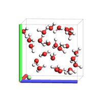
plams.view(box, direction="tilt_x", show_lattice_vectors=True, width=200, height=200)
reference_job = plams.AMSNVTJob(
    settings=reference_settings,
    molecule=box,
    name="amber95_md",
    nsteps=1000,
    timestep=0.5,
    temperature=300,
    thermostat="Berendsen",
    tau=100,
    writeenginegradients=True,
    samplingfreq=100,
)
reference_job.run();
[16.10|12:17:11] JOB amber95_md STARTED
[16.10|12:17:11] JOB amber95_md RUNNING
[16.10|12:17:15] JOB amber95_md FINISHED
[16.10|12:17:15] JOB amber95_md SUCCESSFUL
Import reference results with ParAMS ResultsImporter
Here we use the add_trajectory_singlepoints results importer. For more details about usage of the results importers, see the corresponding tutorials.
QET fine-tuning uses the imported energy and force labels; explicit atomic charges are not required.
importer = ResultsImporter(settings={"units": {"energy": "eV", "forces": "eV/angstrom"}})
importer.add_trajectory_singlepoints(reference_job.results.rkfpath(), properties=["energy", "forces"])
["energy('amber95_md_frame001')",
 "energy('amber95_md_frame002')",
 "energy('amber95_md_frame003')",
 "energy('amber95_md_frame004')",
 "energy('amber95_md_frame005')",
 "energy('amber95_md_frame006')",
 "energy('amber95_md_frame007')",
 "energy('amber95_md_frame008')",
 "energy('amber95_md_frame009')",
 "energy('amber95_md_frame010')",
... output trimmed ....
 "forces('amber95_md_frame002')",
 "forces('amber95_md_frame003')",
 "forces('amber95_md_frame004')",
 "forces('amber95_md_frame005')",
 "forces('amber95_md_frame006')",
 "forces('amber95_md_frame007')",
 "forces('amber95_md_frame008')",
 "forces('amber95_md_frame009')",
 "forces('amber95_md_frame010')",
 "forces('amber95_md_frame011')"]
Optional: split into training/validation sets
Machine learning potentials in ParAMS can only be trained if there is both a training set and a validation set.
If you do not specify a validation set, the training set will automatically be split into a training and validation set when the parametrization starts.
Here, we will manually split the data set ourselves.
Let’s first print the information in the current ResultsImporter training set:
def print_data_set_summary(data_set: Any, title: str) -> None:
    print(f"{title}:")
    print(f"    number of entries: {len(data_set)}")
    print(f"    number of job IDs: {len(data_set.jobids)}")
    print(f"    job IDs: {data_set.jobids}")


print_data_set_summary(importer.data_sets["training_set"], "Original training set")
Original training set:
    number of entries: 22
    number of job IDs: 11
    job IDs: {'amber95_md_frame008', 'amber95_md_frame007', 'amber95_md_frame006', 'amber95_md_frame009', 'amber95_md_frame002', 'amber95_md_frame010', 'amber95_md_frame003', 'amber95_md_frame004', 'amber95_md_frame001', 'amber95_md_frame011', 'amber95_md_frame005'}
Above, the number of entries is twice the number of jobids because the energy and forces extractors are separate entries.
The energy and force extractors for a given structure (e.g. frame006) must belong to the same data set. For this reason, when doing the split, we call split_by_jobid
training_set, validation_set = importer.data_sets["training_set"].split_by_jobids(0.8, 0.2, seed=314)
importer.data_sets["training_set"] = training_set
importer.data_sets["validation_set"] = validation_set

print_data_set_summary(training_set, "Training set")
print_data_set_summary(validation_set, "Validation set")
Training set:
    number of entries: 16
    number of job IDs: 8
    job IDs: {'amber95_md_frame008', 'amber95_md_frame007', 'amber95_md_frame009', 'amber95_md_frame002', 'amber95_md_frame010', 'amber95_md_frame003', 'amber95_md_frame004', 'amber95_md_frame005'}
Validation set:
    number of entries: 6
    number of job IDs: 3
    job IDs: {'amber95_md_frame001', 'amber95_md_frame006', 'amber95_md_frame011'}
Store the reference results in ParAMS yaml format
Use ResultsImporter.store() to store all the data in the results importer in the ParAMS .yaml format:
yaml_dir = Path("yaml_ref_data")
importer.store(str(yaml_dir), backup=False)

for path in sorted(yaml_dir.iterdir()):
    print(path)
yaml_ref_data/job_collection.yaml
yaml_ref_data/job_collection_engines.yaml
yaml_ref_data/results_importer_settings.yaml
yaml_ref_data/training_set.yaml
yaml_ref_data/validation_set.yaml
Set up and run a ParAMSJob for training ML Potentials
See the ParAMS MachineLearning documentation for all available input options.
Select the MatGL backend and the packaged QET-PBE-2025 model to fine-tune QET.
Training the model may take a few minutes.
job = ParAMSJob.from_yaml(str(yaml_dir))
job.name = "params_finetune_qet"
job.settings.runscript.nproc = 1
job.settings.input.Task = "MachineLearning"
job.settings.input.MachineLearning.CommitteeSize = 1
job.settings.input.MachineLearning.MaxEpochs = 250
# job.settings.input.MachineLearning.LossCoeffs.Energy = 10
job.settings.input.MachineLearning.Backend = "MatGL"
job.settings.input.MachineLearning.MatGL.Model = "QET-PBE-2025"
job.settings.input.MachineLearning.MatGL.LearningRate = 0.001
job.settings.input.MachineLearning.MatGL.LearningRateSchedule.Type = "Cosine"
job.settings.input.MachineLearning.MatGL.LearningRateSchedule.FinalFactor = 0.01
job.settings.input.MachineLearning.MatGL.TrainableLayers = "All"
job.settings.input.MachineLearning.Target.Forces.Enabled = "Yes"
job.settings.input.MachineLearning.Target.Forces.MAE = 0.05
job.settings.input.MachineLearning.RunAMSAtEnd = "Yes"
job.run(watch=True);
[16.10|12:17:15] JOB params_finetune_qet STARTED
[16.10|12:17:15] JOB params_finetune_qet RUNNING
[16.10|12:37:17] JOB params_finetune_qet FINISHED
[16.10|12:37:17] JOB params_finetune_qet SUCCESSFUL
Results of the ML potential training
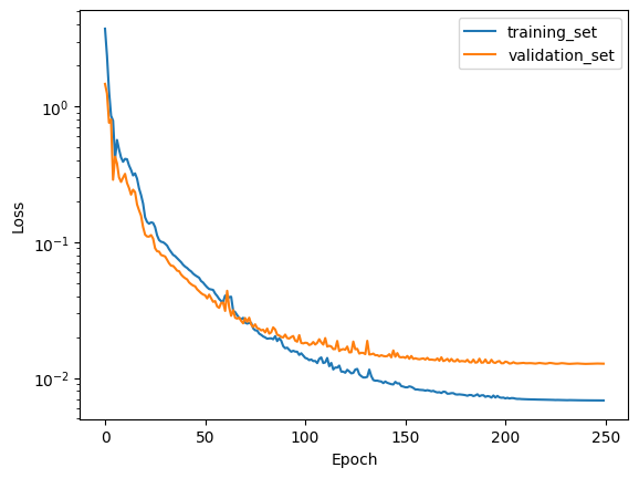
Use job.results.get_running_loss() to get the loss value as a function of epoch:
fig, ax = plt.subplots()
for data_set in ("training_set", "validation_set"):
    epoch, loss = job.results.get_running_loss(data_set=data_set)
    ax.semilogy(epoch, loss, label=data_set)
ax.set_xlabel("Epoch")
ax.set_ylabel("Loss")
ax.legend()
ax;
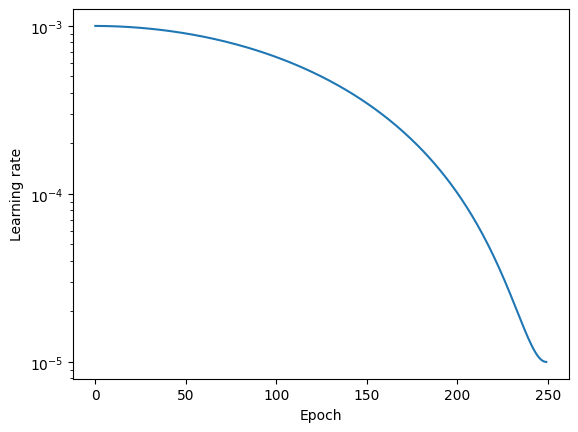
The MatGL results also contain the learning rate used for every epoch. Plot it on a logarithmic scale to verify the cosine schedule:
fit_results = job.results.get_machine_learning_results()[0]
epoch, learning_rate = fit_results.get_learning_rate_history()
fig, ax = plt.subplots()
ax.semilogy(epoch, learning_rate)
ax.set_xlabel("Epoch")
ax.set_ylabel("Learning rate")
ax;
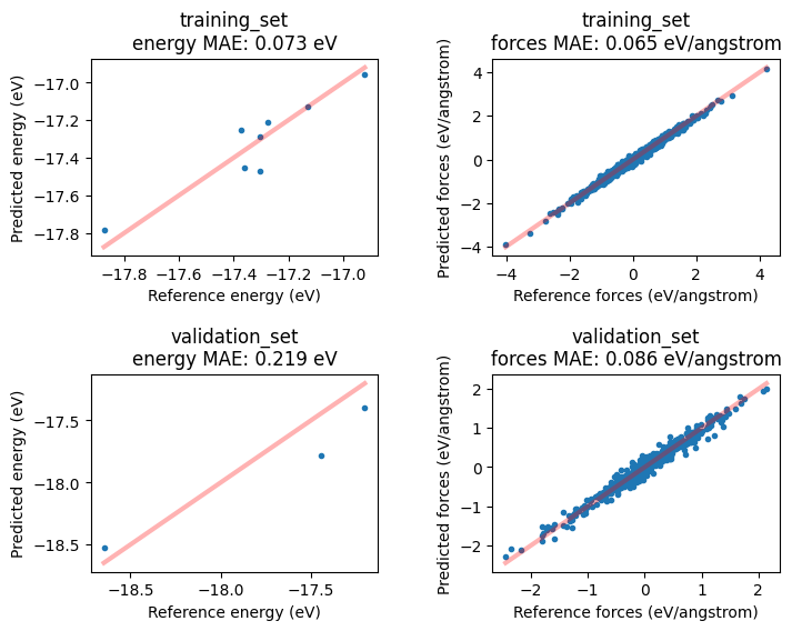
If you set MachineLearning%RunAMSAtEnd (it is on by default), this will run the ML potential through AMS at the end of the fitting procedure, similar to the ParAMS SinglePoint task.
This will give you access to more results, for example the predicted-vs-reference energy and forces for all entries in the training and validation set. Plot them in a scatter plot like this:
fig, axes = plt.subplots(nrows=2, ncols=2, figsize=(8, 6))

for row, data_set in enumerate(("training_set", "validation_set")):
    evaluator = job.results.get_data_set_evaluator(data_set=data_set, source="best")
    for column, key in enumerate(("energy", "forces")):
        data = evaluator.results[key]
        ax = axes[row, column]
        ax.plot(data.reference_values, data.predictions, ".")
        ax.set_xlabel(f"Reference {key} ({data.unit})")
        ax.set_ylabel(f"Predicted {key} ({data.unit})")
        ax.set_title(f"{data_set}\n{key} MAE: {data.mae:.3f} {data.unit}")
        lower = min(min(data.reference_values), min(data.predictions))
        upper = max(max(data.reference_values), max(data.predictions))
        ax.plot([lower, upper], [lower, upper], linewidth=3, alpha=0.3, color="red")

fig.subplots_adjust(hspace=0.6, wspace=0.4)
axes[-1, -1];
Get the engine settings for production jobs
First, let’s find the path to where the fine-tuned QET model resides using get_deployed_model_paths(). This function returns a list of paths to the trained models. In this case we only trained one model, so we access the first element of the list with [0].
The returned path is the path we need to give as the ParameterDir input option in the AMS MLPotential engine. For other backends it might instead be the ParameterFile option.
To get the complete engine settings as a PLAMS Settings object, use the method get_production_engine_settings():
print(job.results.get_deployed_model_paths()[0])

production_settings = job.results.get_production_engine_settings()
print(plams.AMSJob(settings=production_settings).get_input())
/Users/ormrodmorley/Documents/code/ams/amshome_version_bump/userdoc/PythonExamples/mlpotential-train-qet/plams_workdir/params_finetune_qet/results/optimization/matgl/matgl

Engine MLPotential
  Backend MatGL
  Model Custom
  ParameterDir /Users/ormrodmorley/Documents/code/ams/amshome_version_bump/userdoc/PythonExamples/mlpotential-train-qet/plams_workdir/params_finetune_qet/results/optimization/matgl/matgl
EndEngine
Run a production MD simulation with the trained potential
The production simulation uses a Nose–Hoover chain thermostat at 300 K with a 100 fs damping constant.
production_settings.runscript.nproc = 1
production_job = plams.AMSNVTJob(
    settings=production_settings,
    molecule=box,
    nsteps=1000,
    temperature=300,
    thermostat="NHC",
    tau=100,
    samplingfreq=100,
    name="production_md",
    timestep=1.0,
)
production_job.run(watch=True);
[16.10|12:37:18] JOB production_md STARTED
[16.10|12:37:18] JOB production_md RUNNING
[16.10|12:37:18] production_md: AMS 2026.201  RunTime: Oct16-2026 12:37:18  ShM Nodes: 1  Procs: 1
[16.10|12:37:22] production_md: Starting MD calculation:
[16.10|12:37:22] production_md: --------------------
[16.10|12:37:22] production_md: Molecular Dynamics
[16.10|12:37:22] production_md: --------------------
[16.10|12:37:22] production_md:          Step       Time    Temp.         E Pot        Pressure        Volume
[16.10|12:37:22] production_md:                     (fs)      (K)          (au)           (MPa)         (A^3)
[16.10|12:37:22] production_md:             0       0.00     300.      -0.68082        -354.016         792.0
... output trimmed ....
[16.10|12:37:58] production_md:           500     500.00     309.      -0.63567          31.227         792.0
[16.10|12:38:05] production_md:           600     600.00     279.      -0.63139          23.045         792.0
[16.10|12:38:12] production_md:           700     700.00     278.      -0.62899        -879.885         792.0
[16.10|12:38:19] production_md:           800     800.00     309.      -0.63013       -1150.554         792.0
[16.10|12:38:28] production_md:           900     900.00     343.      -0.61720       -1410.246         792.0
[16.10|12:38:36] production_md:          1000    1000.00     347.      -0.61600        -823.229         792.0
[16.10|12:38:36] production_md: MD calculation finished.
[16.10|12:38:36] JOB production_md FINISHED
[16.10|12:38:36] production_md: NORMAL TERMINATION
[16.10|12:38:36] JOB production_md SUCCESSFUL
charges = production_job.results.get_charges(engine="MDStep1000")
print(f"{'Atom':>4}  {'Element':>7}  {'Charge (e)':>12}")
for index, (atom, charge) in enumerate(zip(box, charges), start=1):
    print(f"{index:4d}  {atom.symbol:>7}  {charge:12.6f}")
Atom  Element    Charge (e)
   1       Na      1.059251
   2       Cl     -0.409621
   3        O     -0.691690
   4        H      0.333270
   5        H      0.351332
   6        O     -0.789767
   7        H      0.348186
   8        H      0.361502
   9        O     -0.764171
... output trimmed ....
  65        H      0.340971
  66        O     -0.715169
  67        H      0.341870
  68        H      0.337992
  69        O     -0.743932
  70        H      0.339615
  71        H      0.363953
  72        O     -0.710986
  73        H      0.340634
  74        H      0.370051
Open trajectory file in AMSmovie
With the production trajectory you can run analysis tools in AMSmovie, or access them from Python. See the AMS manual for details.
trajectory_file = production_job.results.rkfpath()
print(trajectory_file)
# !amsmovie "{trajectory_file}"
/Users/ormrodmorley/Documents/code/ams/amshome_version_bump/userdoc/PythonExamples/mlpotential-train-qet/plams_workdir/production_md/ams.rkf
See also
Python Script
#!/usr/bin/env python
# coding: utf-8

# ## Overview
#
# Import reference data from a short trajectory of aqueous sodium chloride, split it into training and
# validation sets, fine-tune the packaged ``QET-PBE-2025`` foundation model with ParAMS,
# and reuse the deployed model in a production MD job.
#
# QET combines an equivariant neural network with charge equilibration, so it can describe charge redistribution without requiring atomic-charge labels during fine-tuning.

from pathlib import Path
from typing import Any

import matplotlib.pyplot as plt
import scm.plams as plams
from scm.base import ChemicalSystem
from scm.inputs import AMS, ForceField
from scm.params import ParAMSJob, ResultsImporter


# ## Run a quick reference MD job for aqueous NaCl
#
# In this example we generate some simple reference data.
#
# If you
#
# * already have reference data in the ParAMS .yaml format, then you can skip this step
# * already have reference data in the ASE .xyz or .db format, you can convert it to the ParAMS .yaml format. See :ref:`convert_params_ase`.

sodium = ChemicalSystem.from_smiles("[Na+]")
chloride = ChemicalSystem.from_smiles("[Cl-]")
water = ChemicalSystem.from_smiles("O")

for system in (sodium, chloride, water):
    system.enable_atom_attributes("forcefield")

sodium.atoms[0].forcefield.type = "IP"
sodium.atoms[0].forcefield.charge = 1.0
chloride.atoms[0].forcefield.type = "IM"
chloride.atoms[0].forcefield.charge = -1.0
water.atoms[0].forcefield.type = "OW"
water.atoms[0].forcefield.charge = -0.834
water.atoms[1].forcefield.type = "HW"
water.atoms[1].forcefield.charge = 0.417
water.atoms[2].forcefield.type = "HW"
water.atoms[2].forcefield.charge = 0.417

reference_settings = plams.Settings()
reference_settings.input = AMS(Engine=ForceField(Type="Amber95"))
reference_settings.runscript.nproc = 1

box = plams.packmol(
    [sodium, chloride, water], n_molecules=[1, 1, 24], density=1.029
)
box = plams.preoptimize(box, settings=reference_settings)
plams.view(box, direction="tilt_x", show_lattice_vectors=True, width=200, height=200, picture_path="picture1.png")


reference_job = plams.AMSNVTJob(
    settings=reference_settings,
    molecule=box,
    name="amber95_md",
    nsteps=1000,
    timestep=0.5,
    temperature=300,
    thermostat="Berendsen",
    tau=100,
    writeenginegradients=True,
    samplingfreq=100,
)
reference_job.run();


# ## Import reference results with ParAMS ResultsImporter
#
# Here we use the ``add_trajectory_singlepoints`` results importer. For more details about usage of the results importers, see the corresponding tutorials.
#
# QET fine-tuning uses the imported energy and force labels; explicit atomic charges are not required.

importer = ResultsImporter(settings={"units": {"energy": "eV", "forces": "eV/angstrom"}})
importer.add_trajectory_singlepoints(reference_job.results.rkfpath(), properties=["energy", "forces"])


# ## Optional: split into training/validation sets
#
# Machine learning potentials in ParAMS can only be trained if there is both a training set and a validation set.
#
# If you do not specify a validation set, the training set will automatically be split into a training and validation set when the parametrization starts.
#
# Here, we will manually split the data set ourselves.
#
# Let's first print the information in the current ResultsImporter training set:

def print_data_set_summary(data_set: Any, title: str) -> None:
    print(f"{title}:")
    print(f"    number of entries: {len(data_set)}")
    print(f"    number of job IDs: {len(data_set.jobids)}")
    print(f"    job IDs: {data_set.jobids}")


print_data_set_summary(importer.data_sets["training_set"], "Original training set")


# Above, the number of entries is twice the number of jobids because the ``energy`` and ``forces`` extractors are separate entries.
#
# The energy and force extractors for a given structure (e.g. frame006) must belong to the same data set. For this reason, when doing the split, we call ``split_by_jobid``

training_set, validation_set = importer.data_sets["training_set"].split_by_jobids(0.8, 0.2, seed=314)
importer.data_sets["training_set"] = training_set
importer.data_sets["validation_set"] = validation_set

print_data_set_summary(training_set, "Training set")
print_data_set_summary(validation_set, "Validation set")


# ## Store the reference results in ParAMS yaml format
#
# Use ``ResultsImporter.store()`` to store all the data in the results importer in the ParAMS .yaml format:

yaml_dir = Path("yaml_ref_data")
importer.store(str(yaml_dir), backup=False)

for path in sorted(yaml_dir.iterdir()):
    print(path)


# ## Set up and run a ParAMSJob for training ML Potentials
#
# See the ParAMS MachineLearning documentation for all available input options.
#
# Select the MatGL backend and the packaged ``QET-PBE-2025`` model to fine-tune QET.
#
# Training the model may take a few minutes.

job = ParAMSJob.from_yaml(str(yaml_dir))
job.name = "params_finetune_qet"
job.settings.runscript.nproc = 1
job.settings.input.Task = "MachineLearning"
job.settings.input.MachineLearning.CommitteeSize = 1
job.settings.input.MachineLearning.MaxEpochs = 250
# job.settings.input.MachineLearning.LossCoeffs.Energy = 10
job.settings.input.MachineLearning.Backend = "MatGL"
job.settings.input.MachineLearning.MatGL.Model = "QET-PBE-2025"
job.settings.input.MachineLearning.MatGL.LearningRate = 0.001
job.settings.input.MachineLearning.MatGL.LearningRateSchedule.Type = "Cosine"
job.settings.input.MachineLearning.MatGL.LearningRateSchedule.FinalFactor = 0.01
job.settings.input.MachineLearning.MatGL.TrainableLayers = "All"
job.settings.input.MachineLearning.Target.Forces.Enabled = "Yes"
job.settings.input.MachineLearning.Target.Forces.MAE = 0.05
job.settings.input.MachineLearning.RunAMSAtEnd = "Yes"


job.run(watch=True);


# ## Results of the ML potential training
#
# Use ``job.results.get_running_loss()`` to get the loss value as a function of epoch:

fig, ax = plt.subplots()
for data_set in ("training_set", "validation_set"):
    epoch, loss = job.results.get_running_loss(data_set=data_set)
    ax.semilogy(epoch, loss, label=data_set)
ax.set_xlabel("Epoch")
ax.set_ylabel("Loss")
ax.legend()
ax;
ax.figure.savefig("picture2.png")


# The MatGL results also contain the learning rate used for every epoch. Plot it on a logarithmic scale to verify the cosine schedule:

fit_results = job.results.get_machine_learning_results()[0]
epoch, learning_rate = fit_results.get_learning_rate_history()
fig, ax = plt.subplots()
ax.semilogy(epoch, learning_rate)
ax.set_xlabel("Epoch")
ax.set_ylabel("Learning rate")
ax;
ax.figure.savefig("picture3.png")


# If you set ``MachineLearning%RunAMSAtEnd`` (it is on by default), this will run the ML potential through AMS at the end of the fitting procedure, similar to the ParAMS SinglePoint task.
#
# This will give you access to more results, for example the predicted-vs-reference energy and forces for all entries in the training and validation set. Plot them in a scatter plot like this:

fig, axes = plt.subplots(nrows=2, ncols=2, figsize=(8, 6))

for row, data_set in enumerate(("training_set", "validation_set")):
    evaluator = job.results.get_data_set_evaluator(data_set=data_set, source="best")
    for column, key in enumerate(("energy", "forces")):
        data = evaluator.results[key]
        ax = axes[row, column]
        ax.plot(data.reference_values, data.predictions, ".")
        ax.set_xlabel(f"Reference {key} ({data.unit})")
        ax.set_ylabel(f"Predicted {key} ({data.unit})")
        ax.set_title(f"{data_set}\n{key} MAE: {data.mae:.3f} {data.unit}")
        lower = min(min(data.reference_values), min(data.predictions))
        upper = max(max(data.reference_values), max(data.predictions))
        ax.plot([lower, upper], [lower, upper], linewidth=3, alpha=0.3, color="red")

fig.subplots_adjust(hspace=0.6, wspace=0.4)
axes[-1, -1];


# ## Get the engine settings for production jobs
#
# First, let's find the path to where the fine-tuned QET model resides using ``get_deployed_model_paths()``. This function returns a list of paths to the trained models. In this case we only trained one model, so we access the first element of the list with ``[0]``.
#
# The returned path is the path we need to give as the ``ParameterDir`` input option in the AMS MLPotential engine. For other backends it might instead be the ``ParameterFile`` option.
#
# To get the complete engine settings as a PLAMS Settings object, use the method ``get_production_engine_settings()``:

print(job.results.get_deployed_model_paths()[0])

production_settings = job.results.get_production_engine_settings()
print(plams.AMSJob(settings=production_settings).get_input())


# ## Run a production MD simulation with the trained potential
#
# The production simulation uses a Nose--Hoover chain thermostat at 300 K with a 100 fs damping constant.

production_settings.runscript.nproc = 1
production_job = plams.AMSNVTJob(
    settings=production_settings,
    molecule=box,
    nsteps=1000,
    temperature=300,
    thermostat="NHC",
    tau=100,
    samplingfreq=100,
    name="production_md",
    timestep=1.0,
)
production_job.run(watch=True);


charges = production_job.results.get_charges(engine="MDStep1000")
print(f"{'Atom':>4}  {'Element':>7}  {'Charge (e)':>12}")
for index, (atom, charge) in enumerate(zip(box, charges), start=1):
    print(f"{index:4d}  {atom.symbol:>7}  {charge:12.6f}")


# ## Open trajectory file in AMSmovie
#
# With the production trajectory you can run analysis tools in AMSmovie, or access them from Python. See the AMS manual for details.

trajectory_file = production_job.results.rkfpath()
print(trajectory_file)
# !amsmovie "{trajectory_file}"