TD-CDFT Response Properties For Crystals (OldResponse)
BAND can calculate response properties such as the frequency-dependent, dielectric function within the theoretical framework of time-dependent current density function theory (TD-CDFT).
This introductory tutorial will show you how to:
- Set up and run a BAND singlepoint calculation (using ADFJobs and ADFInput)
- Set up and run a BAND TD-CDFT, linear response calculation (using ADFJobs and ADFInput) with the
OldResponsemethod - Visualize the dielectric funtion using ADFSpectra
If you are not at all familiar with our Graphical User Interface (GUI), check out the Introductory tutorial first.
Step 1: Create the system
We now want to create a silicium-diamond crystal. Let us import the geometry from our database of structures:
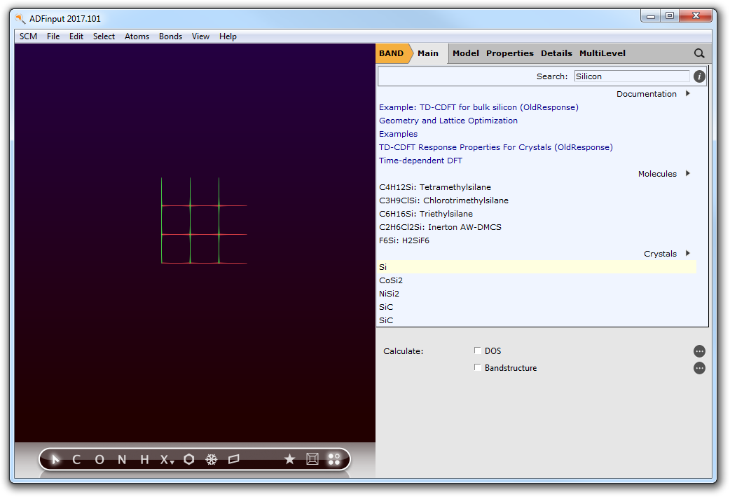
- 1. Open ADFinput.2. Switch from ADF to BAND.3. Search for Silicon in the search box (magnifying glass).4. Select Crystals → Si.
Step 2: Run a Singlepoint Calculations (LDA)
To get an estimate regarding the error in the band-gap energy of LDA for Si diamond, we shall run a single-point calculation first.
Attention
To enhance the speed of the calculation, we will neglect a convergence study w. r. t. kspace sampling and basis set.
- 1. Select the ‘BAND Main’ panel.2. Change Basis set to DZP.3. Check the Bandstructure and DOS boxes.
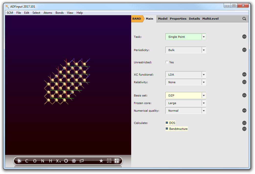
- 4. Go to Details → Integration K-Space.5. Set the K-Space option for pre-2014 defaults to 3.

- 6. File → Save As..., use name LDA_SP.adf7. File → Run
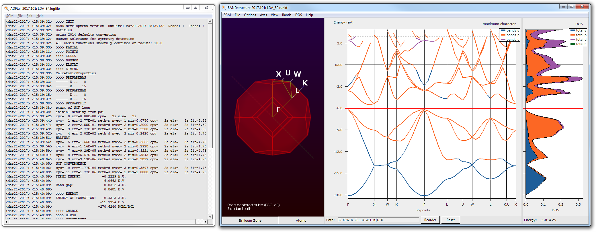
After the calculation finished, we can check the band-gap energy e.g. in the logfile. Furthermore, with the help of the BandStructure module we can validate that a very basic property is reproduced by this rather poor k-space sampling - Si diamond has an indirect band-gap.
- 8. SCM → Logfile9. SCM → Bandstructure
Step 3: Run an OldResponse Calculation (ALDA)
We can now start the calculation of the frequency-dependent, dielectric function with the help of linear response TD-CDFT.
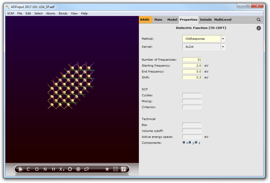
In the previous step we learned that the calculated band-gap for the chosen theoretical level is approx. 0.85 eV. This is approximately 0.3 eV below the experimental band-gap. Hence, we will shift the virtual crystal orbitals by this value in energy space. As a reasonable frequency range will sample from 2.0 eV to 5.0 eV with step-size of 0.1 eV.
- 1. Go to the ‘BAND Main’ panel and uncheck the Bandstructure and DOS boxes.2. Go to Properties → Dielectric Function (TD-CDFT).3. Change Method to OldResponse.4. Change Number of frequencies to 31.5. Change Starting frequency to 2.0.6. Change End frequency to 5.0.7. Change Shift to 0.3.
- 8. File → Save As..., use name LDA_TDCDFT.adf9. File → Run
After the calculation finished, we can analyse the calculated dielectric function by plotting it with ADFspectra.
- 10. SCM → Spectra11. File → TD-CDFT → Dielectric Function → XX
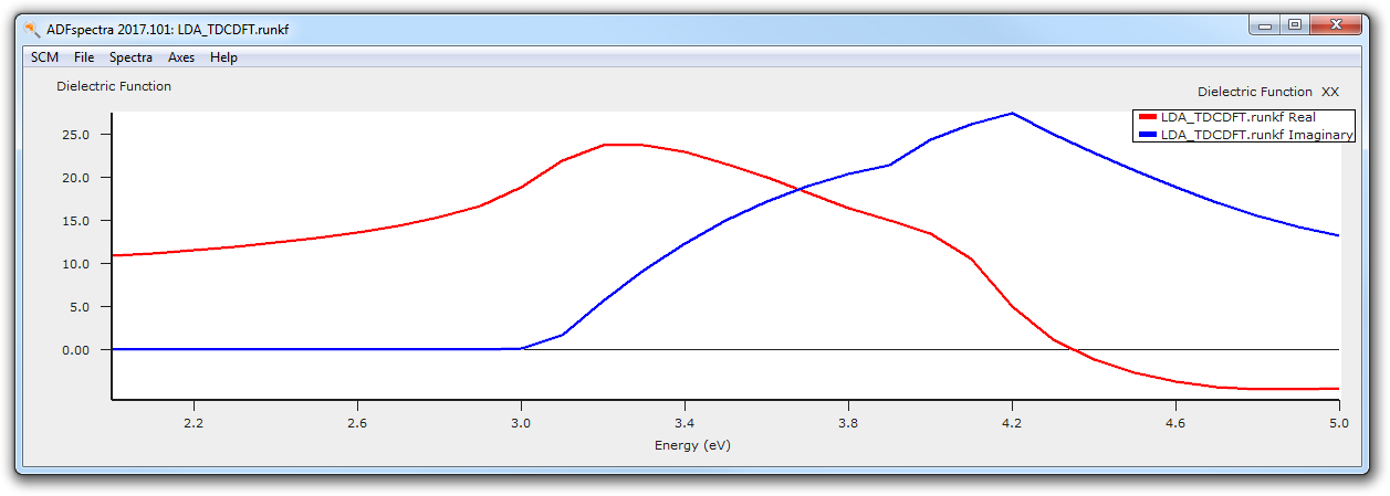
The general features of the frequency-dependent dielectric function are nicely reproduced, but for a quantitatively better result one has to converge the k-space sampling, basis set and real-space sampling. Also switching to the Berger2015 kernel would improve the results further. [Ref]