Burning methane

This tutorial will help you to:

• create a simple mixture (methane and oxygen)
• set up to burn it quickly (set up your ReaxFF simulation)
• burn it: perform the actual ReaxFF simulation
• visualize what is happening during and after the simulation
• extract a reaction network from the trajectory

Step 1: Start ReaxFFinput

Start ADFjobs

SCM → New input

Switch to ReaxFF mode (panel bar ADF → ReaxFF)

Step 2: Create a methane / oxygen mixture

Next we will make the methane - oxygen mixture. For full combustion we need at least 2 oxygen molecules for each methane molecule. So we will use 100 methane molecules and 250 oxygen molecules.

Edit → Builder

The Builder allows you to build your system, and set some things like the cell vectors that define the computation cell.

Note

ReaxFF always uses periodic boundary conditions. The default cell is a cube with sides of 100 Angstrom. The cell is located around the atoms already present, or in the default location for the current method if no atoms are present yet (for ReaxFF in the positive quadrant, for BAND around the origin).

You can use the Builder to add many molecules, randomly distributed. In the list of molecules to be added the Current molecule is already present. If you have any molecules already, the new molecules will be added. Right now we have no molecules yet, so we can remove that entry.

Click on the - button in front of Current

Click the + button in front of Molecules once (so now we can specify two kinds of molecules to add)

Enter 25 on the diagonal to change the box to a cube of 25.0 Angstrom

Click in the entry field of the first line

Type me to search for methane

As you can see, a search box appears to find your molecule, very similar to the search box in the panel bar.

Select the Methane (ADF) match

Click the file select button on the other ‘Fill box with’ line

Click in the entry field of the second line

Type o to search for O2

Select the O2 (ADF) match

Change the 100 copies of O2 into 250 copies

You now have specified how the builder should build your system: 100 methane molecules with 250 oxygen molecules added.

At the bottom of the Builder panel you can see that the current density is zero. The new density, after adding methane and oxygen, will be around 1 g/mL, which is obviously very high for this mixture. For this tutorial that is fine as it means things will happen faster.

Next we will actually generate the molecules:

Click the Generate Molecules button

The molecules are generated at random positions and orientations, with constraint that all atoms (between different molecules) are at least the specified distance (2.5 Angstrom) apart.

The system looks good, we can now close the Builder:

Click the Close button at the bottom of the Builder window

Step 3: Prepare for burning: set up the simulation

The next step is to set up the details of the simulation.

Note

For this tutorial we will perform an MD simulation, at very high temperature and density. This is to make things happen quickly. Obviously it is not a realistic system.

Click the i on the right side of the Force field line

A new window should appear describing what force fields are available, including a short description and references. For this particular example we will use the CHO force field for hydrocarbon oxidation.

Close the window describing the force fields

Click on the folder icon next to Force field

Select the CHO.ff force field

Enter 50000 as number of iterations

Enter 10000 as number of non-reactive iterations

From the menu Method choose NVT Nose-Hoover chains

Specify a temperature of 3500 K

Note

We will be using the Nose-Hoover thermostat which yields better overall sampling results in general. The Nose-Hoover damping constant is dependend on the system size because ideally it should match the period of the internal oscillations of the system. In the present case we stick to the default value of 100 fs but one might want to test different values in a realistc setup.

To setup a Nose-Hoover thermostat with a damping constant of 100 fs:

Select NVT Nose-Hoover chains from the menu Method

Specify a temperature of 3500 K

Step 4: Burn it: run the simulation

Now we will run your set-up:

Use the File → Run command

When asked to save your input, save it with the name Methane

ADFjobs should come to the foreground, and your job should be visible at the top. On the right side you can see that the job is running (this is indicated by the gear-icon). When running, in the ADFjobs window the progress of your simulation is showing (from the logfile). When you click on the progress lines the logfile will open in its own window:

Click on the logfile lines in the ADFjobs window to open the logfile

As you can see in the logfile, the simulation is running.

To see more details, we now will use ADFmovie. Note that you can do this while the simulation is still running!

Start ADFmovie: SCM → Movie in the logfile window

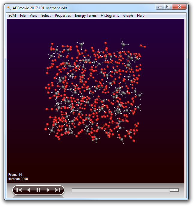
ADFmovie will show you the trajectory of your system. Note that it will automatically read new data as soon as it becomes available.

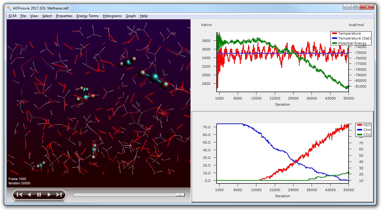
It can also show graphs of the properties that ReaxFF calculates:

In the ADFmovie window:

Use the Properties → Temperature command

Use the Properties → Temperature (Set) command

Use the Properties → Potential Energy command

Note that the two temperatures (the actual temperature, and the set temperature) are both plotted on one axes. The other axes is used for the second property (in this case the potential energy).

You can go to a particular point in the simulation using the slider below the window showing your system, or you can click somewhere on one of the curves plotted. You can also use the arrow keys (left and right) to move through the simulation.

Tip

Click on the temperature curve to move around in the movie. Jump to the end of the movie to follow the progress

As ReaxFF is a reactive force field, reactions may take place. In this particular example the methane should react with the oxygen, eventually producing H2O and CO2.

You can make graphs that show how many of the different molecule types are present. The following instructions often work, but it depends on what molecules are present in your simulation. You might try this step again after waiting some time. Remember that we requested 10000 non-reactive iterations, so just leave it running for 15000 iterations or so. Especially the production of H2O and CO2 take some time.

After about 15000 iterations:

Use the Properties → Molecule Fractions command

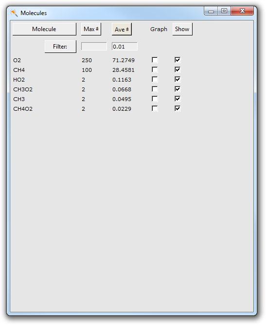
In the dialog window that appears all molecules that occur in the calculation are shown (up to the moment the dialog is created). By clicking at the top in the dialog you can sort the molecules by name, occurrence in the last frame, or average occurrence.

The first column of check boxes allow you to select for which molecules to show a graph of their occurrence (the number of molecules of the selected type, per time step).

The second column allows you to show or hide that particular molecule type. This can be convenient to hide the original molecules for example, so you can easily see what is happening.

The two text entry fields at the top are thresholds used to filter the number of species shown. In this particular tutorial they are not needed, all molecule types are visible. But if you are dealing with a system with many thousands of species the dialog would otherwise no longer be usable. Obviously you can adjust the filter values to your needs, and reapply them by clicking the Filter button.

In the molecule fractions dialog:

Check the graph check box to show the curve for H2O

Repeat for CH4, and for CO2 if any present yet.

Obviously, no reactions take place in the first 10000 iterations.

Tip

You can drag the legend in the plotting area around with the mouse

You can put one of the curves on a different axes if you wish:

Click once on the curve showing the number of CH4 molecules, this makes it the ‘active’ curve

Use the Graph → Curve On Right Axes command

Clicking on the curve also had two other effects (besides making it the active curve): you jumped to the iteration in the movie corresponding to the point where you clicked, and the molecules that belonged to that curve are selected.

Flying to the selection also makes it easier to spot them:

Use the Properties → Molecule Fractions command to add a CO2 curve if you have not yet done so

Click on the curve showing the CO2 production

Use the View → Molecule → Balls And Sticks to view the CO2 molecules more easily

Use the View → Fly To Selection command a few times

When you now go forward or backwards in time, it is easier to see how the reactions actually take place. Note that the atoms remain selected, even if they are no longer part of a CO2 molecule. In a similar way you can focus on H2O produced:

Switch back wireframe: View → Molecule → Wireframe

Click on the curve showing the H2O production

Use the View → Fly To Selection command if needed

Use the View → Molecule → Balls And Sticks to view the H2O molecules more easily

Another tool to see what is going on is hiding molecule that are not of interest. In this example, let’s hide CH4 and O2:

Clear the selection by clicking in empty space

Switch to wireframe: View → Molecule → Wireframe

In the molecule fractions dialog, uncheck the second check box for CH4 (in the Show column)

In the molecule fractions dialog, uncheck the second check box for O2 (in the Show column)

Use the molecule fractions dialog to show all molecules again

Wait until the calculation is ready

Select the CO2 curve (click on it)

Move it to the left axes: Graph → Curve On Left Axes

There is another tool to focus on a region of interest, by showing only some selected part:

View → Molecule → Ball ; sticks

Select an atom somewhere in the center

Use the Select → Within radius ... command, and select all within 5 Angstrom

View → Show Selection Only

Click in empty space to clear the selection

View → Show All to see everything again

Step 5: Analyze it: Create a reaction network

In this part of the tutorial we will analyze our methane trajectory in more detail by creating a reaction network using the automated reaction event detection (ChemTraYzer) in ADFmovie.

Note

A ChemTraYzer analysis can currently not be performed on periodic systems, e.g. surfaces. If the molecules created during the reaction exceed a size of ~50 atoms, the 2D depiction of the species can fail. If this happens, it is still possible to obtain results when running the analysis from the command line. See how to run on the command line .

Properties → Reaction Event Detection

The dialog window coming up displays the settings for the reaction event detection. It consists of two steps, a processing and an analysis step, both of which have different settings. In short, the processing step will determine which species are formed at what time, while the analysis step creates a reaction network and calculates the rate constants.

For now, we just stick to the default values:

Click on Process

this will start both the processing and the analysis step. Depending on the size of the trajectory this can take some time (a few minutes on a modern desktop computer). You can follow the progress messages in the bottom right of the dialog window. Once the message “Ready” appears, the calculation is finished:

In the bottom panel of the ChemTraYzer dialog you will now find the total number of reactions and species as obtained during the processing step and the filtered number of reactions and species as obtained during the analysis step.

Click on Browse

Your Browser will open and display an overview page of the ChemTraYzer results:

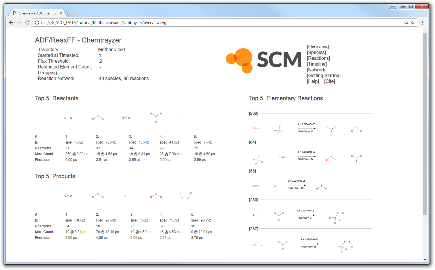
Step 6: Analyze it: Browse a reaction network

The results can be explored by clicking on molecules or one of the links on the top right next to the SCM logo. You can use the same links or your browser history (\(\leftarrow\)) to return to a previous page.

Let’s start by taking a look at the reactions of one of the most reactive species, e.g. the methyl radical:

Click on the image of the CH3 radical listed under “Top 5 Reactants”

You will see the results for the methyl radical, i.e. all reactions it is involved in:

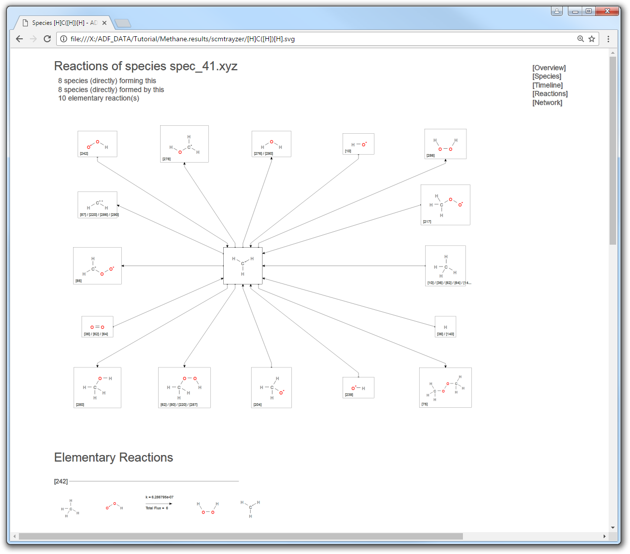
Clicking again on the central species will now direct you to the Cartesian coordinates. Depending on your browser settings these will be displayed by an external program, e.g. an editor, or inside your browser:

The arrows connecting the species indicate whether they contribute to the formation or decrease of the central species while the numbers label the index of the corresponding elementary reaction.

Note

If you are using Microsofts Internet Explorer (IE10 or IE11) you will only see lines instead of arrows. This is due to a bug in Internet Explorer that is unlikely to be fixed. Using any other browser will resolve this.

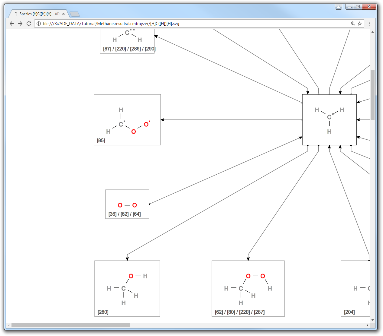
For example: The O2 molecule contributes to the formation of methyl radicals via elementary reactions #36, #62 and #64:

If you scroll down you will find a listing of all elementary reactions the methyl radical is involved in. The label “Total Flux” indicates how often the reaction was observed during the simulation time whilst the rate constant refers to the forward reaction:

Next we take a look at all species found by the reaction detection

Use your browser (\(\leftarrow\)) to navigate back to the overview page

Click on [Species] next to the SCM logo on the top right

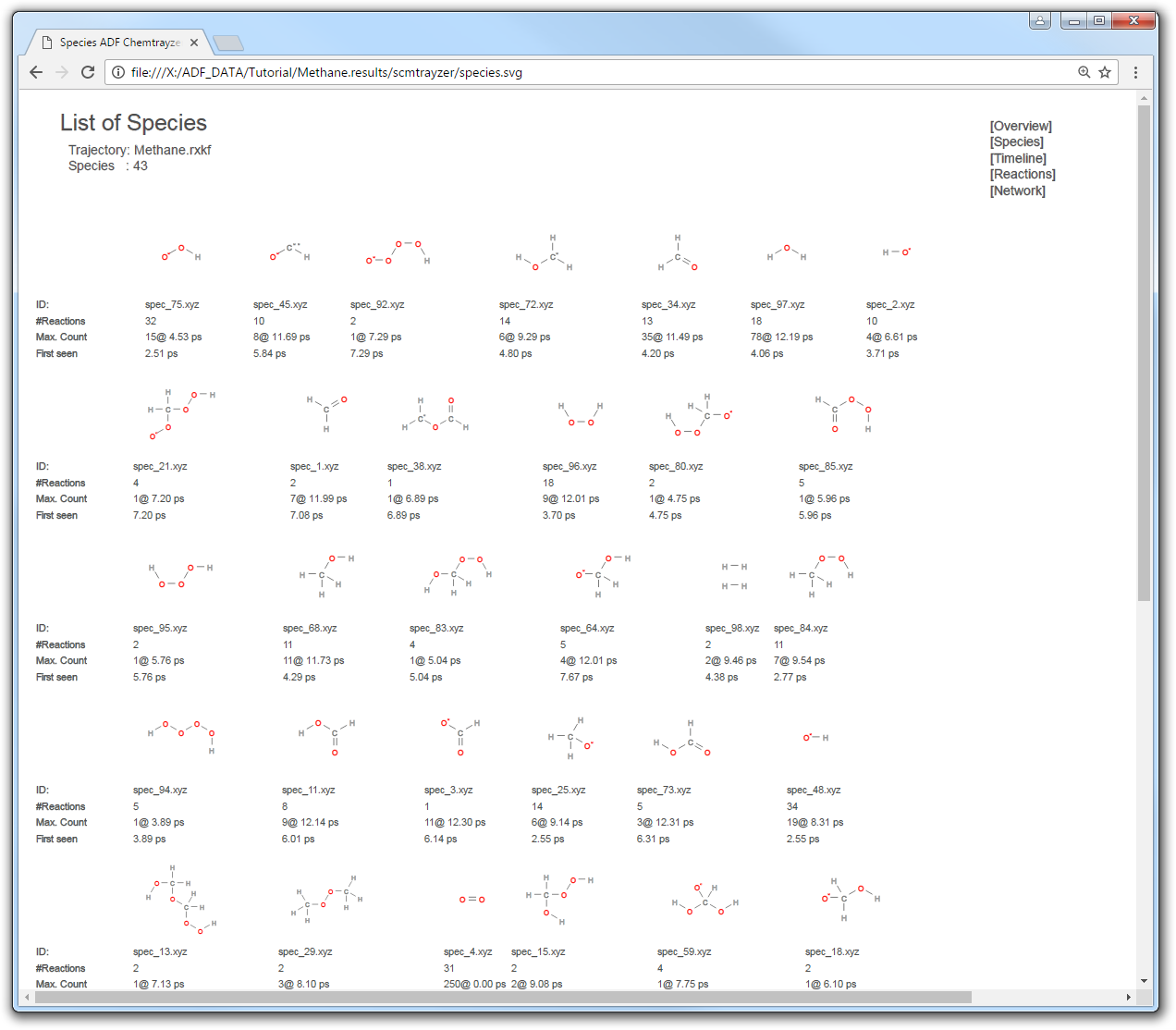
You will see a list of all species with some information on when the species was first observed, how many reactions it is involved in and finally the maximum concentration of the species:

Clicking on [Reactions] will show a similar overview for all elementary reactions, while [Timeline] will bring up a timeline visualizing the species’ first appearances during the trajectory.

You can also take a look at the complete reaction network:

Click on [Network] on the top right

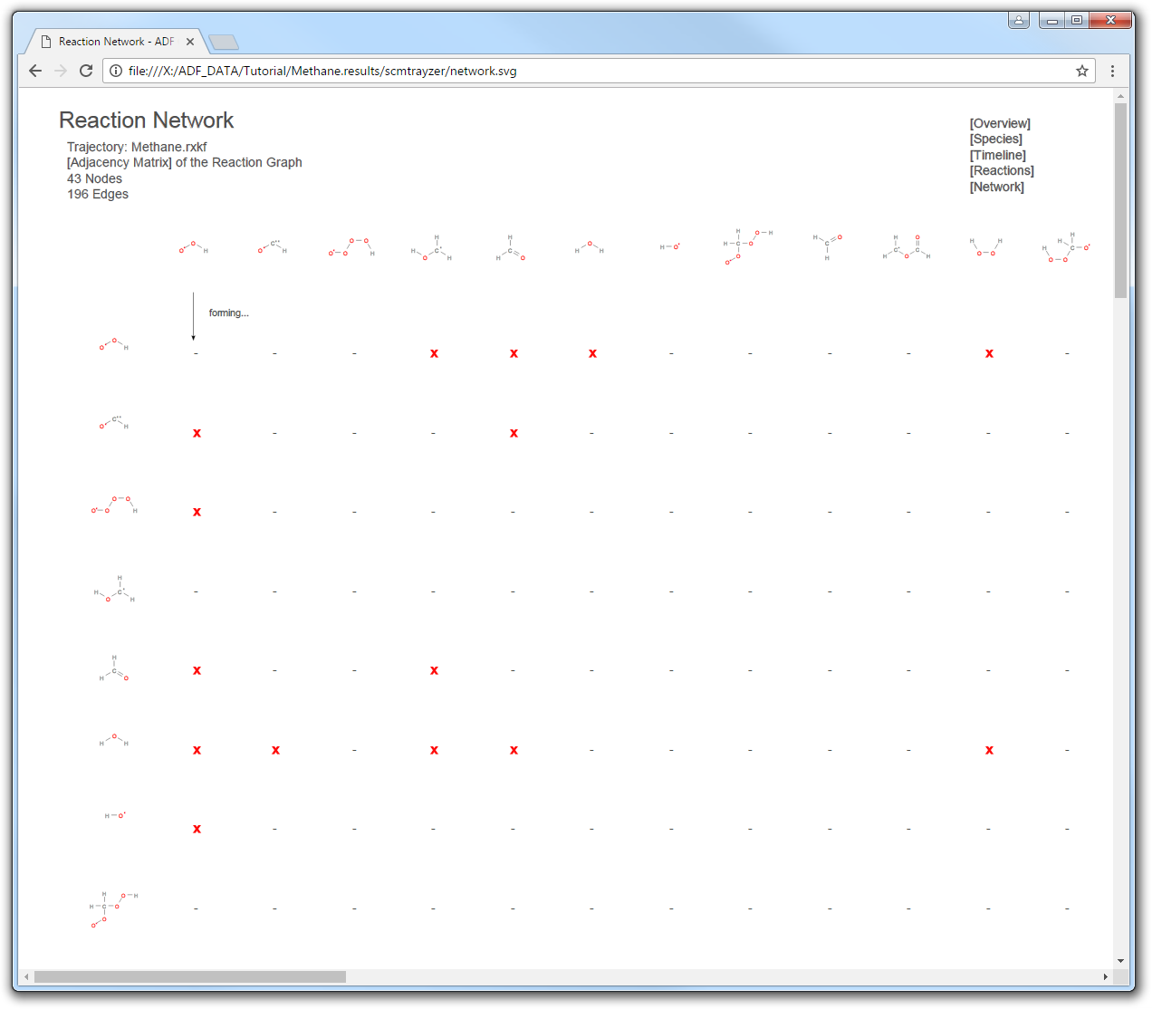
A graphical representation of the adjacency matrix, illustrating the connections between the species, is shown. In this matrix, a column represents a “forming” relation, while a row represents a “formed by” relation. For example, methanol (CH3OH, 1st column) forms water (H2O, 2nd row), while methanol itself can also be (re)-formed or formed by, e.g. hydrogen peroxide (HOOH, 11th column vs. 1st row).

While scrolling in and out of the adjacency matrix, you might have already realized that even our medium sized reaction network can be quite confusing and hard to oversee. However, the amount of species can easily be reduced by applying filters to the reaction network as described in the next section.

Step 7: Analyze it: Filter a reaction network

For now, let’s assume we are interested in oxidized carbohydrates only and want to filter the reaction network due to that constraint:

Bring up the ChemTraYzer dialog from ADFmovie

Set the Flux Threshold to 2

Select O from the Restrict Element Count menu and enter 1-2

Select O from the Group Species by Atom dropdown menu

Click Analyze and wait for the analysis to finish

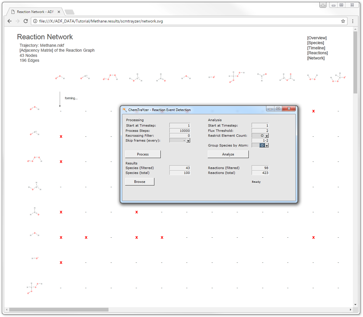
Note that we do not need to re-run the processing step but can now run the analysis directly. By choosing the above settings we will only consider elementary reactions that occur at least twice (“Flux Threshold = 2”), contain species with one or two oxygen atoms (“Restrict Element Count”) and sort the species according to the amount of oxygen they contain (“Group Species by Atom”).

Once the analysis has finished:

Refresh your Browser or click Browse in the ChemTraYzer dialog

The species displayed in the list of species all contain at least one but not more than two oxygen atoms and are sorted:

To prepare for the next tutorial, quit everything:

Bring the ADFjobs window to the foreground

Use the SCM → Quit command to close all windows for this job