Bands, DOS, and the Fermi surface
In this tutorial we consider a metallic system for which the spin-orbit effect is important.
The system under study is cubic TlBi. As both Tl and Bi are heavy elements we use the Spin-Orbit level for relativity. As this is a metal we also take a look at the fermi surface.
Step 1: Load the geometry
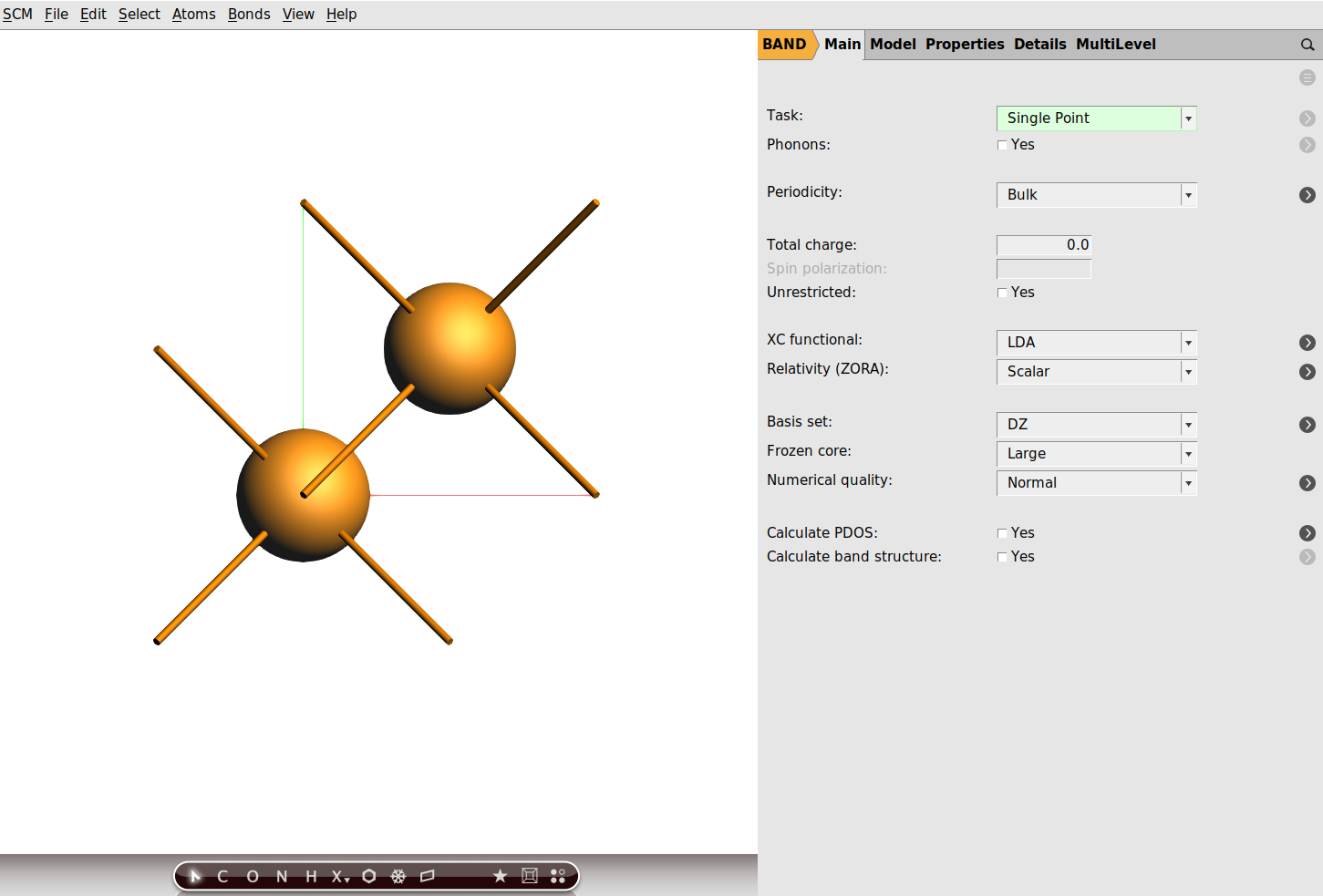
Here we will use the standard geometry as it is available from AMSinput.

The editor should now show the atoms of the first unit cell as well as the lattice vectors:
Step 2: Calculation
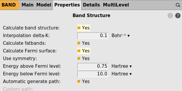
With the system loaded it is time to setup the calculation
Yes next to Calculate PDOS and Calculate band structure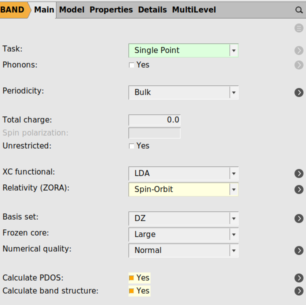
BandsDosFermiSurface.amsNow run the calculation with File → Run. This calculation may take a few minutes.
Note
The results shown here have been calculated with k-space quality good. This is normally recommended for metallic systems. In this case, however, the band structure is almost unaffected.
Step 3: Inspecting the results
After the calculation is complete, open the results with SCM → Band Structure
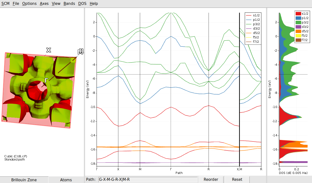
In the picture the default ranges for the DOS axis have been changed to better see the partial DOS contributions.
Once you have achieved this there are a few interesting things to observe. First of all you see a list of angular momentum labels. While normally these are “s,p,d,f”, now there are more choices due to the spin-orbit coupling. All levels (except for s) have been split in two. For instance the p shell is split into a p1/2 and a p3/2 level. This is true both for the “fat band” coloring of the band structure curves, and the (partial) dos contributions.
You can also see that the fermi level (horizontal black line) crosses some bands, and we are dealing with a metal.
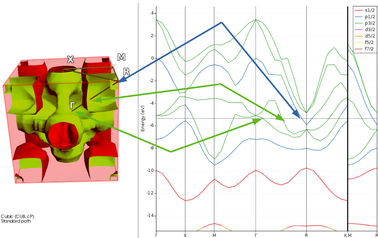
Another interesting thing is that in the left most panel the Fermi surface is shown.
All the three the parts, from left to right: Fermi surface, Band Structure and DOS are related.
The DOS at a certain energy can be regarded as a sum of the band structure plot, counting the crossings at that energy. The purple colored peak at -18 eV is clearly caused by the equally purple band.
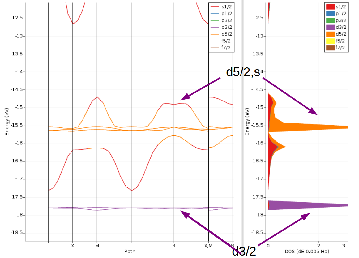
So both the bands and DOS at this energy have mostly a d3/2 character. This band has very little dispersion, and it is almost core like. A bit higher in energy we find the d5/2 band which is more diffuse and shows more dispersion. It also mixes a bit with s functions.
The fermi surface is an implicit surface defined by where any band has an energy exactly equal to the fermi energy. From the central panel we can see that on the path from Gamma to R there are three bands crossing the fermi level. Two are colored green, and hence of the P3/2 character, while the other one is blue, and of the P1/2 character.