PEDA-NOCV - decomposing the orbital relaxation term
This tutorial will teach you how to perform a Periodic Energy Decomposition Analysis (PEDA) combined with the Natural Orbitals for Chemical Valency (NOCV) method for periodic systems with BAND. It will also show how to visualize NOCV orbitals and NOCV deformation densities.
Setting up the System and the Calculation
Preparations for the PEDA-NOCV calculation
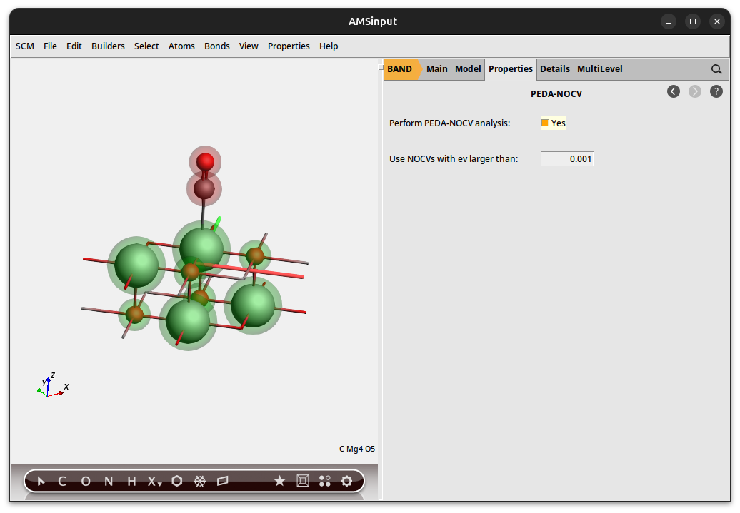
Now the PEDA-NOCV has to be switched on. Go to the PEDA-NOCV menu,
You can define a NOCV eigenvalue threshold (default: 0.001) which handles the amount of output.
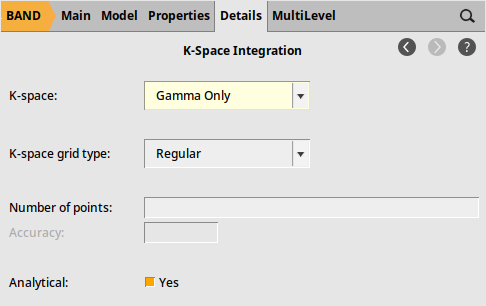
Keep in mind that the PEDA-NOCV is implemented for \(\Gamma\)-only systems. So, go to the ‘Integration K-Space’ menu,
Save and run the calculation
Now you can save and run the calculation.
Step 2: Checking the results
After the calculation of the fragments and the PEDA are finished you can look for the PEDA results. Therefore, open the “Output” using the SCM dropdown menu.
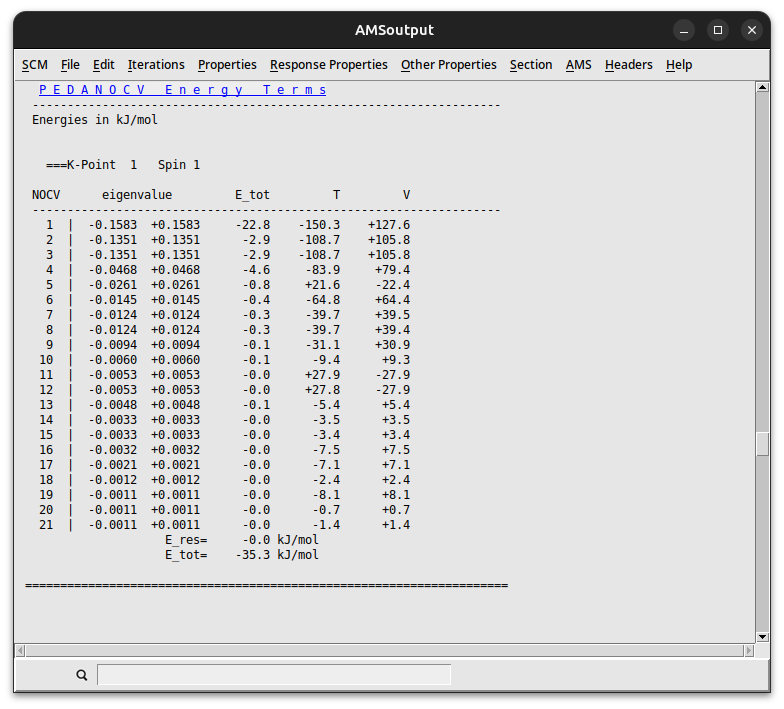
You can jump to the ‘PEDA-NOCV Energy Terms’ via the corresponding button in the ‘Properties’ drop-down menu.
Reference results:
Step 3: Plotting NOCV orbitals and deformation densities
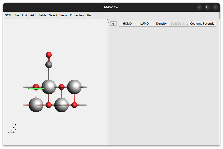
You can visualize the charge NOCV deformation densities which describe the charge flow between the fragments. Therefore, open the “View” using the SCM drop-down menu.
Depending on your preferences (w.r.t. showing atoms of neighboring cells) you will end up with the following representation of AMSview.
Step 3a: Plotting NOCV deformation densities
We will now visualize some NOCV deformation densities
 → Isosurface: With Phase
A table will appear which will let you select the NOCV deformation density.
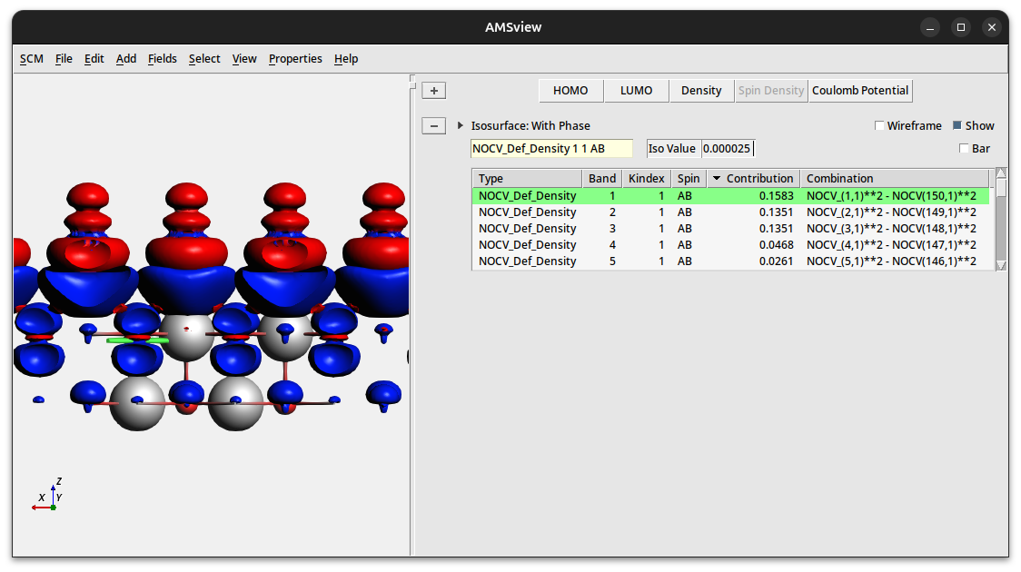
According to the information in the “NOCV Def Densities” table, the first NOCV deformation density is a combination of NOCV orbital 1 (the first term denotes the donor/occupied NOCV) and 150 (the second term denotes the acceptor/unoccupied NOCV). This deformation density visualizes the charge flow from red to blue lobes. Here, the charge transfer from the CO to the MgO surface is shown.
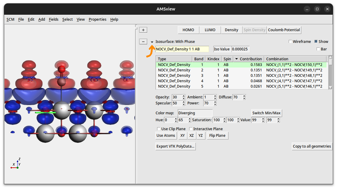
You can toggle extra visualization options by clicking on the tiny arrow next to “Isosurface: With Phase”:
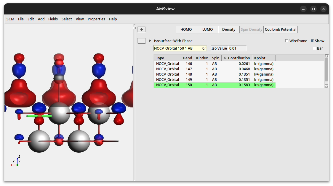
Step 3b: Plotting NOCV orbitals
These NOCV orbitals can be visualized by changing the field to ‘NOCV Orbitals’.
Selecting the 1st and 150th NOCV orbitals will trigger the calculation of their isosurfaces. The orbitals can then be visualized one at a time. (Or you can add a second isosurface to show both of them.)
NOCV orbital 1 shows predominantly a lone-pair localized at the CO fragment (note: the iso value is set to 0.01)
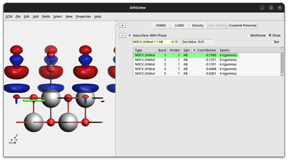
NOCV orbital 150 shows predominantly a lobe connecting the CO fragment with a Mg atom of the surface.