A relative energy gradient (REG) analysis along a PES Scan (1D)¶

Overview¶

In this tutorial, we present a Relative Energy Gradient (REG) analysis 1-2 based on a QTAIM/IQA energy decomposition. This REG analysis is capable of selecting energy terms such that they reflect the overall energy variations of the system. This is a crucial feature for gaining meaningful chemical insights from an energy partitioning method, such as IQA in this case. The efficacy of the method was originally demonstrated by the Poperlier’s group in Manchester using the B3LYP-level description of the water dimer 1. It was shown that a selected subset of energy terms can provide a semi-qualitative description of the system’s behavior. Importantly, the method is based on physically meaningful principles and does not require any prior knowledge of the system or arbitrary parameters. Overall, the REG analysis offers a reliable and intuitive metric for analyzing energy partitioning in chemical systems.

Note

Using this script for published research requires citing the original REG paper 1. Please note that another Python script (not compatible with ADF however) has been developed by Popelier’s group under a MIT license. It is freely available here

Contents of this tutorial:

Setting up a PES Scan (1D) and QTAIM/IQA parameters to run an ADF calculation that determines and saves IQA descritors at each converged geometry.
Performing a subsequent REG analysis using a Python/PLAMS script that extracts IQA results along the reaction path.
Interpreting REG results (water dimer, example taken from the original paper).

This tutorial assumes a basic familiarity with the GUI. If you are not familiar with using the GUI yet, you might take a look at the GUI introduction tutorials before continuing.

Note

The ADF calculation we are going to run in this tutorial takes approximately half an hour on a modern desktop computer (2023).

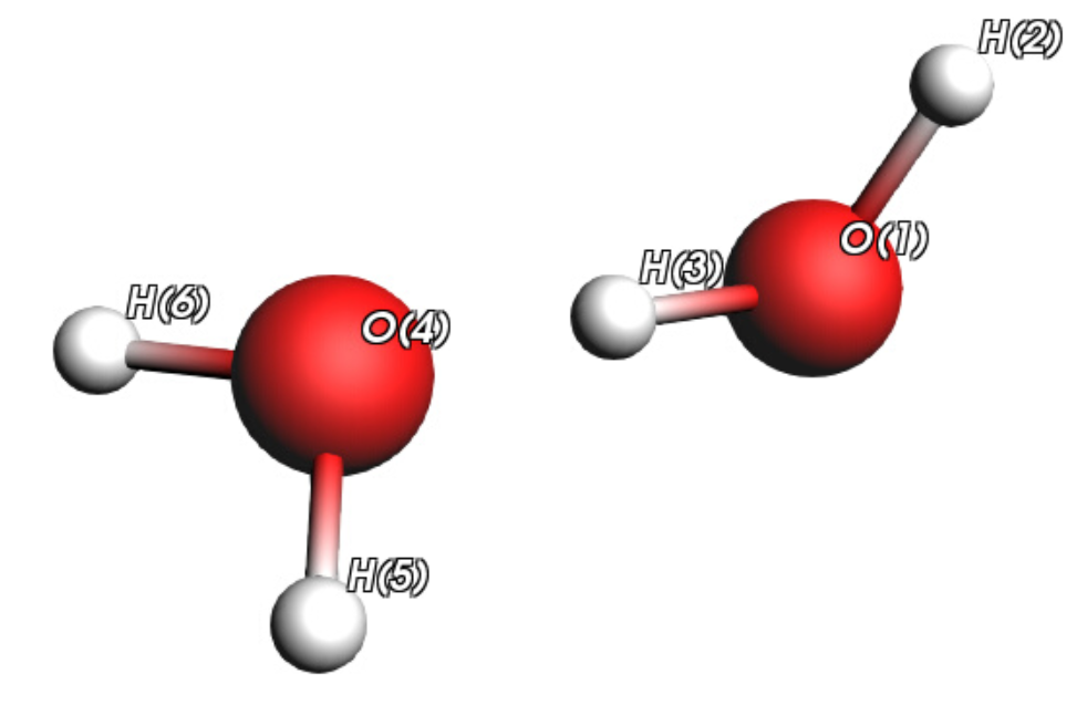
The System¶

This tutorial studies a very simple system: two water monomers in their most stable dimer conformation as illustrated on this picture.

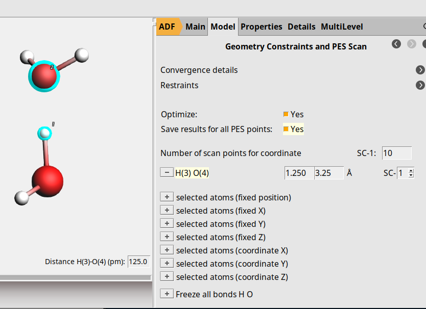
In the original paper, a PES Scan was first performed in 10 steps along the O…H hydrogen bond (from 1.25 Å to 3.25 Å) at the B3LYP/aug-cc-pVTZ level. You can find more details in Reference 1.

In this tutorial, we want to keep the same protocol. We will then choose the B3LYP functional and an equivalent STO basis set (TZ2P).

Importing the initial structure and setting the job parameters¶

You can download the initial structure from this XYZ file (or construct it directly on screen if you are familiar with the GUI building tools). In this file, we kept the same atom numbering with respect to Popelier’s original paper.

Download the XYZ file by clicking here
In AMSinput: File → Import Coordinates
Select the XYZ file you just downloaded using the file dialogue window

Now we can set the parameters for the PES Scan:

Select Task → PES Scan
On the right, click on 
In the new panel, tick the Results for all PES points check box
Select the two atoms of the hydrogen bond by keeping the shift key pressed
Click now on the  sign next to O(4)…H(3) (path coordinate)
Check the initial value is set to 1.25 Å and set the final value to 3.25 Å

Your PES Scan settings should now correspond to this screen capture:

Now, follow the following steps for the QTAIM/IQA settings:

Switch to the QTAIM panel: Properties → QTAIM
In this new panel, tick the Perform QTAIM analysis check box
Select Full for the analysis level
Tick the Interacting Quantum Atoms (IQA) check box
Check if the verbose print mode is selected (that should be selected by default)

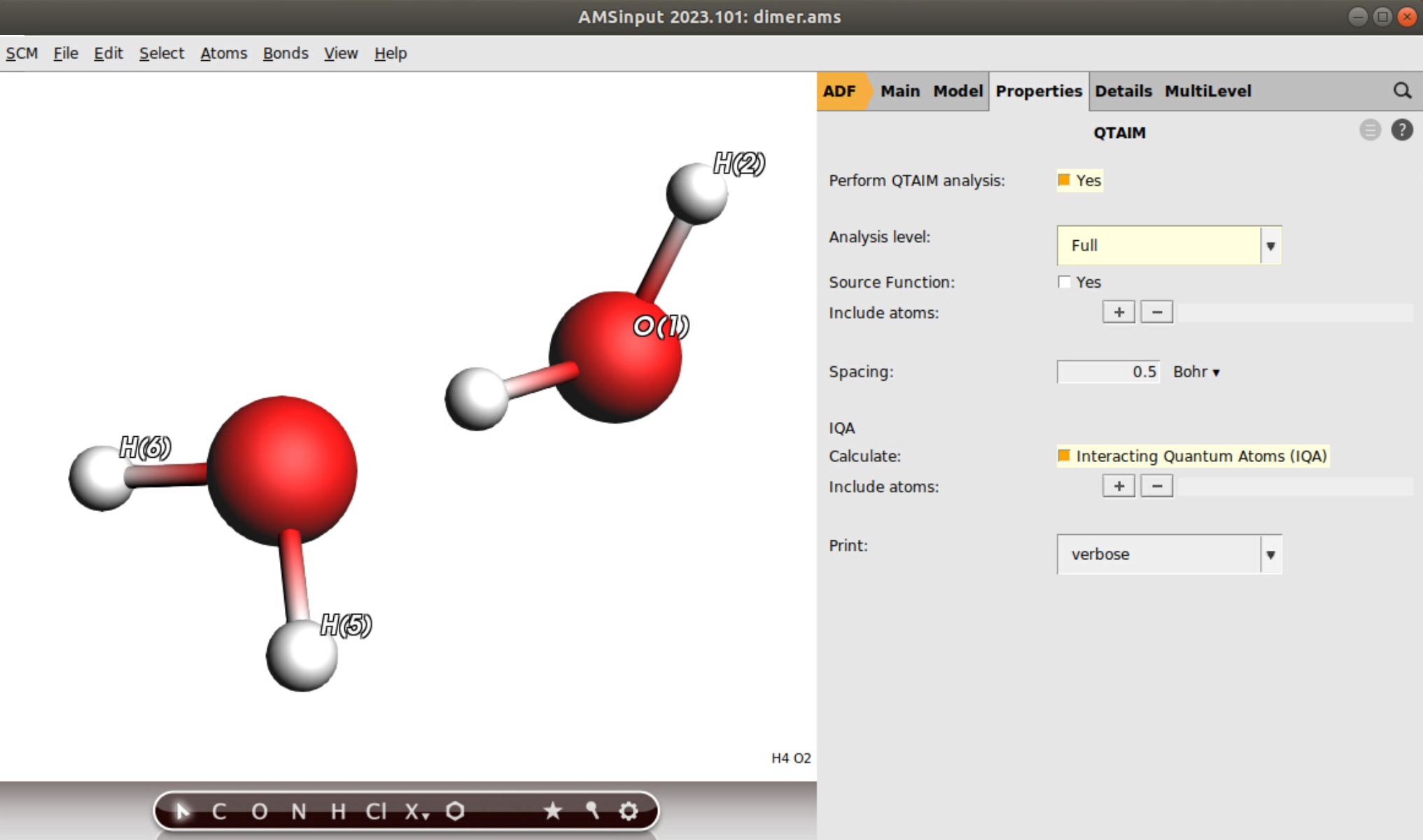
Finally, set the last general settings:

Switch back to the Main panel
Select the B3LYP XC functional
Select None for Relativity
Choose the TZ2P basis set and no frozen core
Let the Numerical Quality on Good for this tutorial

Note

Please note that we always recommend a high quality integration grid for IQA calculations (good or even very good/Excellent).

Performing the PES Scan and the REG analysis¶

Save the settings and run the ADF calculation.

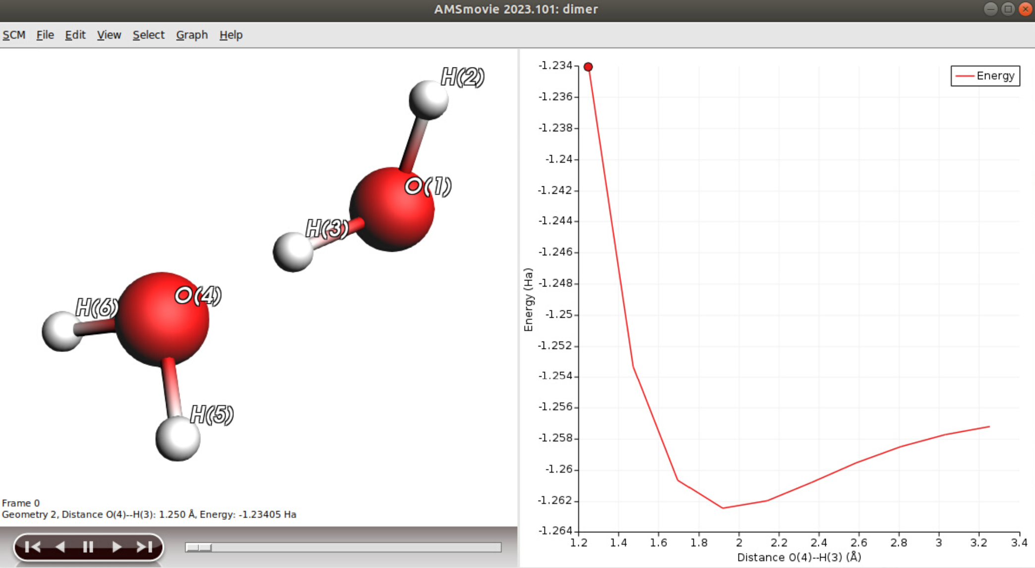
At the end of the calculation, we recommend to check the PES Scan in AMSMovie: SCM → Movie The total bond energy profile should be similar to the one we obtain on this picture:

You can now quit ADF (you do not need to save the changes): SCM → Quit All.

To perform the REG analysis, you need to download our Python/PLAMS script here. This script has been tested with AMS2023 and should be compatible with later versions. You can now execute it using the following command:

$AMSBIN/plams REGScan.py -v resultsdir=path_to_your_results_directory

For instance, if your AMS input was named dimer.ams, a dimer.results folder has been created. Consequently, we use the following command:

$AMSBIN/plams REGScan.py -v resultsdir=./dimer.results

Eventually, we obtain two output files: dimer_REGScan.txt and dimer_REGScan.csv. The first one contains the main REG results and the second one all the data needed for a post treatment with a spreadsheet.

Script Troubleshoot¶

If the script does not run properly, please check the following points:

Check the AMS version (2023 or later).
Check the name and the path of your results directory in the command line. You must not forget to add -v resultsdir=path_to_your_results_directory. See the example above.
Check if all the needed python libraries are installed (edit the script to find the required libraries).
Check if you did not forget to save the converged points of your PES Scan: Model → Geometry Constraints and PES Scan.
In Details → Run Script, check if the runscript auto update check box is ticked.
If you cannot find the problem, please contact support@scm.com.

Interpreting the results¶

1) Extracting chemical information from the PES Scan¶

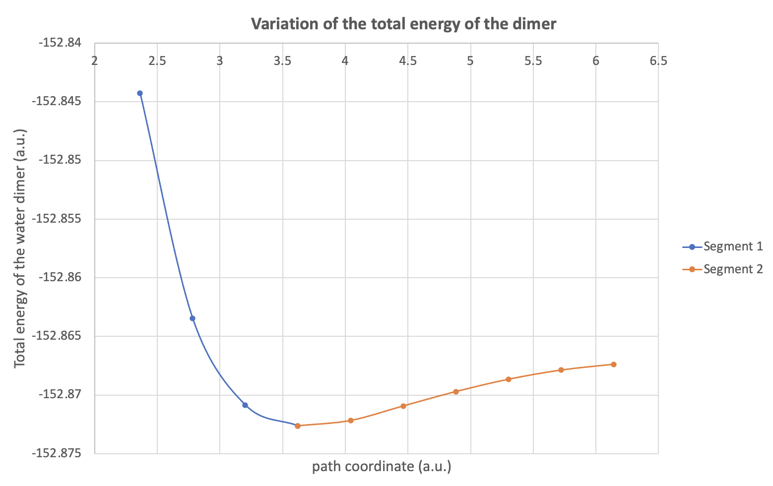
The energetic profile is usually divided in several parts (segments), according to the extrema values of the total energy. In our example, our Morse potential exhibits a single minimum at 1.917 Å (hydrogen bond length). Therefore, we obtain two segments (see Fig. 5 in the original paper), the first one corresponding to a path coordinate varying from 1.250 Å to 1.917 Å while the total energy decreases and the second one to a path coordinate varying from 1.917 Å to 3.250 Å while the dimer dissociates towards a total energy corresponding to the sum of the two isolated fragment energies. The following (Excel) graph illustrates this segmentation along the path coordinate. You can plot it easily by importating all the data in Excel with the second CSV output file (see part 2 below).

This first version of the REGScan script examines the variations of each IQA intra-atomic energy (Eintra) as well as IQA inter-atomic interaction energies (either VCl or VX for Coulomb and exchange parts respectively) along each segment. Then, a linear regression is performed for each of these IQA descriptors with respect to the variation of the total energy (or the total bond energy; only the intercept value will change). $m_{REG,i}$ corresponds to the slope of each linear regression equation (one per IQA descriptor):

\[E_i(s) = m_{REG,i} \cdot E_{total}(s) + c_i\]

where $E_{i}(s)$ corresponds to the values of each IQA descriptor i along the path coordinate (s) and $E_{total}(s)$ corresponds to the values of the total energy along the path (or, again, the total bond energy since only the $c_i$ will differ).

For each segment of the path, all the results of this REG analysis are saved in the first output textfile (job_name_REGScan.txt).

A positive $m_{REG}$ value (with a high value of R² or Pearson coefficient r) corresponds to a descriptor variation that correlates to the total energy variation and contributes positively to this variation. More precisely, if $m_{REG}$ is greater than 1, the corresponding descriptor varies more rapidly than the total energy while a $m_{REG}$ value inferior to 1 corresponds to a descriptor that varies more slowly than the total energy.

In this table (see job_name_REGScan.txt for details), you find the positive $m_{REG}$ values as well as statistical measures for the first segment (sorted in decreasing order).

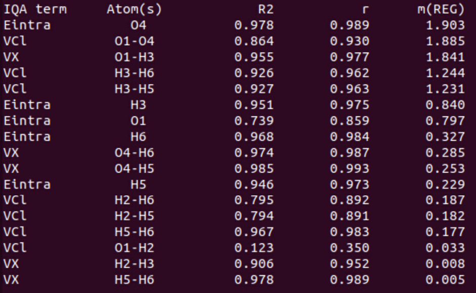
We clearly see that the first barrier (when shortening the O…H bond distance, compressing the dimer) is partly due to the increase of the Eintra(O4) energy term with the largest $m_{REG}$ coefficient (1.903). This is in agreement with a recent paper 2 showing that steric repulsions correspond to an increase of intra-atomic energy terms. To a lesser extent, the H3 intra-atomic term is also correlated (R² = 0.951) to the total energy variation with a $m_{REG}$ value close to 1 (0.840). The second source of repulsion is the electrostatic repulsion VCl between O1 (HB donor) and O4 (HB acceptor). This is in agreement with the chemical intuition allowing to expect a stronger repulsion between two negatively charged atoms when the distance decreases. However, we note that this term does not perfectly correlates with the total energy variations (R² = 0.864). Finally, we observe that H3 and H5 repel each other strongly (as well as H3 and H6) when the inter-fragment distance decreases too much. These terms also contribute to the barrier with a R² coefficent greater than 0.92 and a m_REG value greater than 1. Finally, the exchange (VX) between O1 and H3 decreases a lot at short distance (this O-H bond begins to break), contributing strongly ($m_{REG}$ = 1.841) to the overall destabilization of the dimer.

In the second part of the table, we find the values for the negative $m_{REG}$ coefficients with the corresponding statistical coefficients, sorted by decreasing absolute values.

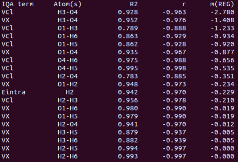
The first terms of this list correspond to the IQA terms that work against the variation of the total energy. The main term ($m_{REG}$ = -2.780 with R² = 0.928) corresponds to the coulombic interaction between O3 and H4 (hydrogen bond). Indeed, decreasing the distance between these atoms increases dramatically the attractive interaction between them. This stabilizes the dimer and counters the global destabilization. To a lesser extent, this hydrogen bond becomes stronger in terms of exchange (covalency). This term varies faster and against ($m_{REG}$ = -1.408) the total energy, tempting to stabilize the dimer. Other terms may also be of interest but some others are meaningless due to poor correlations with the total energy variations (R² < 0.9; VCl(O1/H3) for instance) or slow variations ($m_{REG}$ close to zero).

A similar analysis can be carried out on the second segment. You can find all the corresponding $m_{REG}$ values as well as R² and Pearson coefficients in the same output file. Besides, a complete analysis of these segments can be found in the original work of Thacker and Popelier.

2) Plotting the variations of IQA descriptors¶

The second output file is a CSV file (spreadsheet) with all data separated with commas (job_name_REGScan.csv). It contains the following values:

the values of the path coordinates (all segments) in the first column.
the values of the total bond energies along the path.
the values of the total energies along the path.
the values of each intra-atomic energy along the path (one per column).
the values of each VCl inter-atomic term along the path (one pair per column).
the values of each VX inter-atomic term along the path (one pair per column).

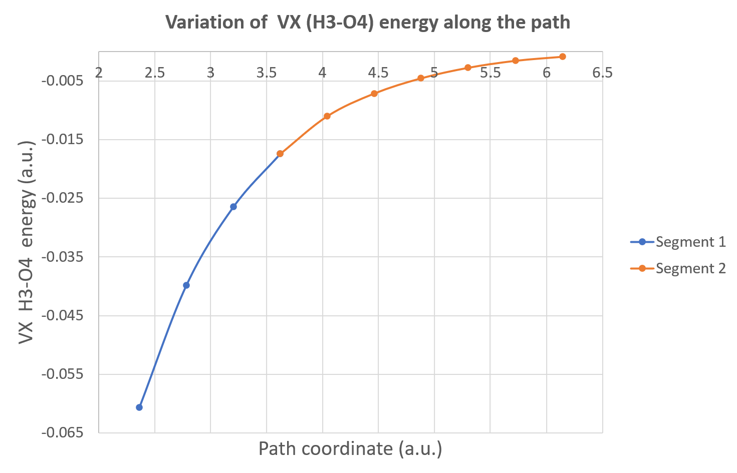
Now, you can plot, for instance, the variation of the inter-atomic exchange energy between H3 and O4 (hydrogen bond). With Excel, we obtain this Figure:

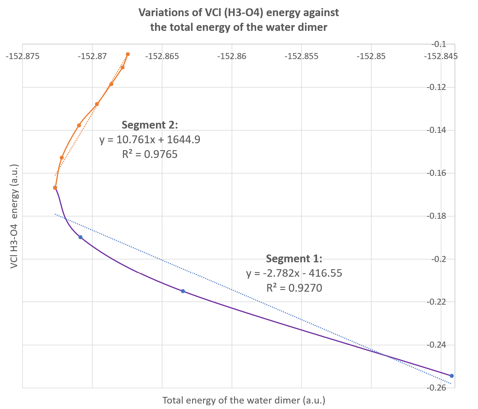
Alternatively, these data can be used to plot the variations of one IQA energetic descriptor against the total energy of the system as illustrated on the figure below. This is called a REG GRAPH, exhibiting the correlations between the two energies for each segment of the path.

It corresponds to the Fig.4 (bottom graph) in the original paper: VCl(H3-O4) with respect to the total energy of the dimer. We added the regression equations on each segment of the graph.

References

1(1,2,3,4): Thacker, J.C.R., Popelier, P.L.A., The ANANKE relative energy gradient (REG) method to automate IQA analysis over configurational change, Theoretical Chemistry Accounts, 136, 86 (2017)
2(1,2): Symons, B., Williamson, D.J., Brooks, C.M., Wilson, A., & Popelier, P.L.A., Does the Intra-atomic Deformation Energy of IQA Represent Steric Energy?, ChemistryOpen 8, 560 (2019).