Restart the DOS or band structure with BAND

It is quite likely that you did a calculation, but forgot to request the DOS or BandStructure. Or maybe you did but want to use different settings.

Fortunately it is possible to calculate these directly from the previous calculation.

With the restart of the DOS it is possible to calculate the DOS with a finer k-space sampling. In this example we first show an example where the DOS does not match the band structure. This missing DOS problem can be solved by simply using a better k-grid. However, it can also be solved by doing a restart, using only a better k-grid for the DOS calculation.

Step 1: Load the geometry

The have the geometry stored as an xyz file

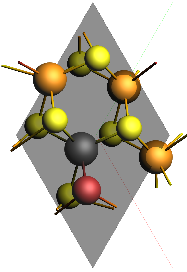
Download CsPbBr3_NR.xyz

Let us load it into AMSinput.

Start AMSinput

File → Import Coordinates…

Select the downloaded file Mo3WSeS7.xyz and click OK

The structure is a MoS2 slab with some substitutions

Step 2: Calculation

With the system loaded it is time to setup the calculation

In the Main panel:

Tick Yes next to Calculate PDOS and Calculate band structure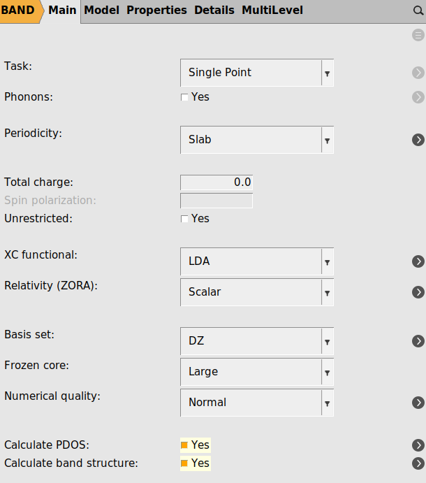

File → Save As…

Save e.g. under test_k=normal.ams

Now run the calculation with File → Run. This calculation may take a few minutes.

Step 3: Inspecting the results

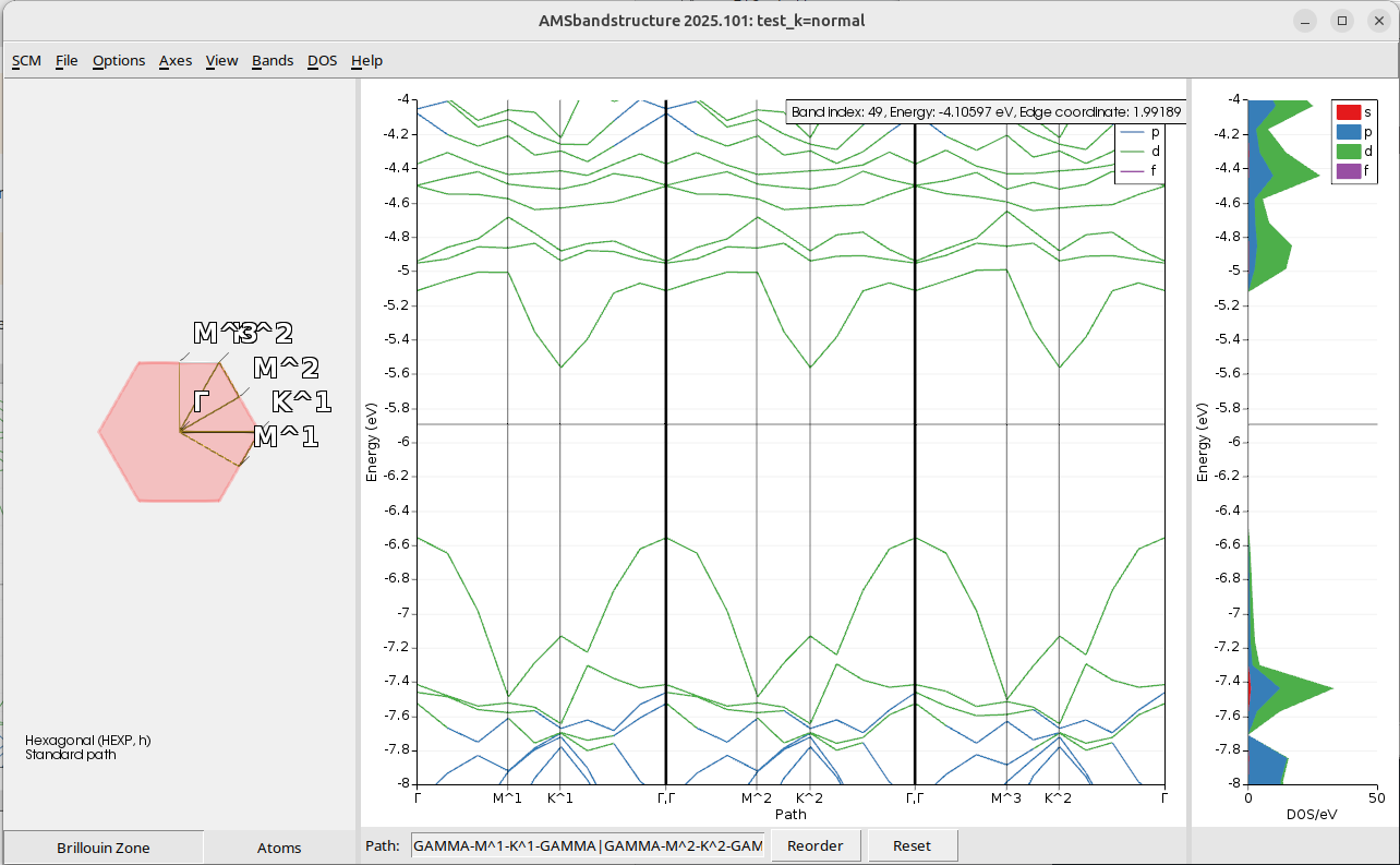
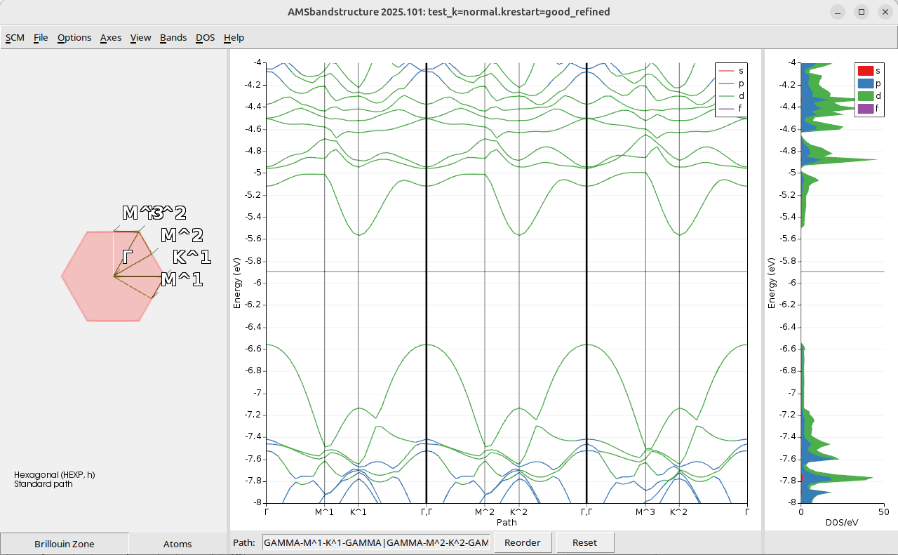
After the calculation is complete, open the results with SCM → Band Structure. To highlight the missing DOS problem change the y-range to -0.3 to -0.1 Hartree

Double click on the “DOS/Ha” axis of the DOS plot

Set the range from 0 to 1000

Double click on the “Energy (Ha)” axis of the DOS plot

Set the range from -0.3 to -0.1

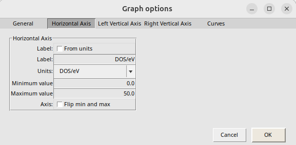
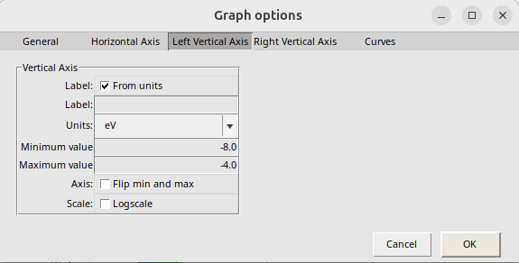
Now we can see the problem: there clearly is a band between -0.20 and -0.19 Hartree, but the DOS is zero in this range.

Step 4: The simple solution: more k-points

The simple solution is to do the whole calculation with a better k-grid.

File → Save As…

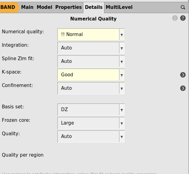
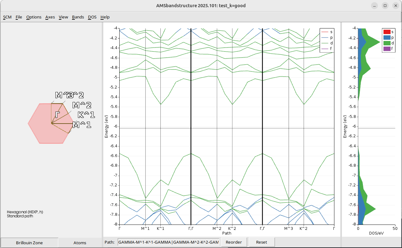
Save e.g. under test_k=good.ams

Run the calculation with File → Run, and this calculation will take a bit longer than before.

Open with amsbands

Modify the DOS plot axes as before

and now there is no longer DOS missing in the -0.20 to -0.19 energy range.

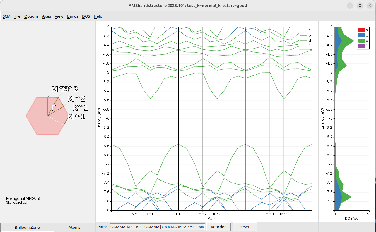
Step 5: Restarting the DOS with more k-points

Open test_k=good.ams

Go to the Details → Restart Details panel and check DOS and band structure

Select the file to restart from test_k=normal.results/band.rkf

File → Save As…

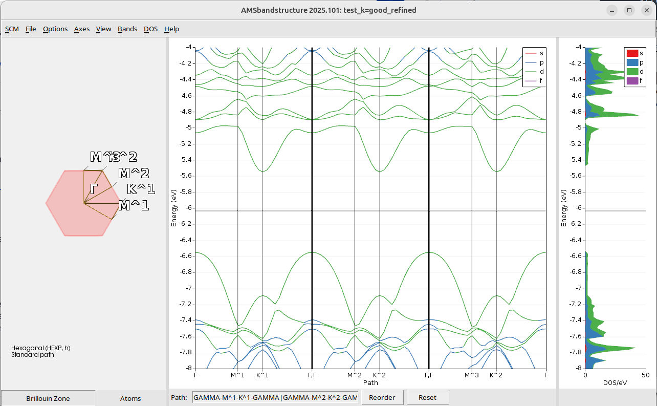
Save e.g. under test_k=normal_krestart=good

Run the calculation

After the calculation is finished open it with amsbands

Change the x-range to 0,1000 and the y-range to -0.3,-0.1

The band structure and DOS look very similar to what we had with a good k-grid for the whole calculation (see Step 4), but obtained in a faster way, avoiding the need to do a full SCF with the good k-grid. Note that there is no longer missing dos between -0.20 and -0.19 Hartree.

Step 6: Refining the plot

In the final step we use more energy points for the dos grid and finer sampling of the band structure

Open test_k=normal_krestart=good.ams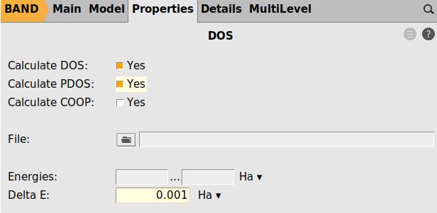

Go to Properties → DOS panel and change the energy interval (delta E) to 0.001

Go to Properties → Band structure panel and change the interpolation delta-K to 0.03

Save as test_k=normal.krestart=good_refined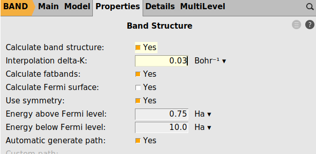

The refined plot is

The reference result obtained by simply doing a full SCF with good k-grid and refined DOS DeltaE and BandStructure delta-K is

and the results look very similar, so you do not need to perform this calculation.