Interacting Quantum Atoms (IQA)¶

This tutorial will show you how to perform interacting quantum atoms calculations with two simple examples: water and PF₅ . You will run them and check the results in the output files.

Step 1: Build H₂O¶

Start AMSinput.
Add an oxygen atom using O tool then add the hydrogens (ctrl/cmd + E).
Choose the Geometry Optimization task in main section.
Set Relativity: None, Basis set: DZP, and Frozen core: None.
Save and Run.

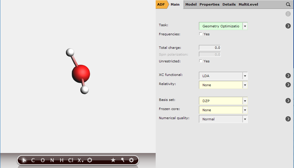
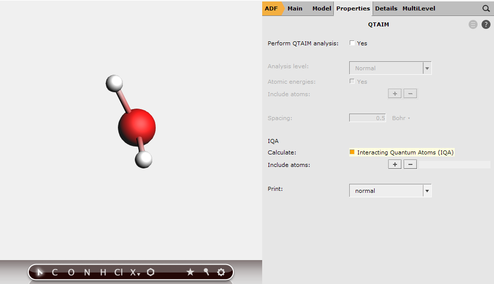
At the end of the calculation, AMSinput will ask whether to use the new coordinates.

Check the Restart engine with engine results check-box.

Select Yes, new job. This creates a new job with the optimized geometry. The SCF will be restarted from the converged solution. Check that the correct restart file is given under Model → Restart.

Step 2: Calculate all interactions in H₂O¶

Choose the Single Point task in main section.
In the panel bar, select Properties → QTAIM.
Check the Calculate Interacting Quantum Atoms (IQA) check-box.
Save again and Run.

Step 3: Analyze the results¶

When the calculation has finished, check the results:

Open the output file: SCM → Output .

Go to the IQA section of the output (Properties → Interacting Quantum Atoms (IQA) ).

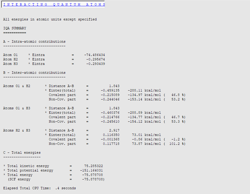
All results are expressed in a.u. unless otherwise specified (for example, kcal/mol). By default, in addition to intra-atomic (‘self’) terms, the total interatomic interaction energy, its covalent and non-covalent parts are printed for each atom pair.

For instance, the total interaction energy between O1 and H2 atoms should be close to -288 kcal/mol at this level of theory (LDA/DZP/Normal Grid). The ‘covalent’ part (exchange) is equal to -135 kcal/mol (47% of the total energy) while the electrostatic contribution (‘ionic part’) corresponds to -153 kcal/mol (53% of the total energy).

It is interesting to note that the repulsive H2-H3 interaction is quite large (73 kcal/mol), due to substantial QTAIM charges on hydrogen atoms (+0.55 e- for each hydrogen). The classical Coulomb part of the energy (+ 74 kcal/mol) is larger than the total interaction energy, explaining why the energy percentage is greater than 100%. It is in fact counterbalanced by stabilizing but rather small exchange energy (less than 1 kcal/mol, consistent with the non-bonded character of the interaction). Finally, we can notice that the electrostatic contribution can be roughly estimated by a point charge model (with QTAIM charges) and Coulomb’s law q(H2) x q(H3) / rH2-H3 » 64 kcal/mol.

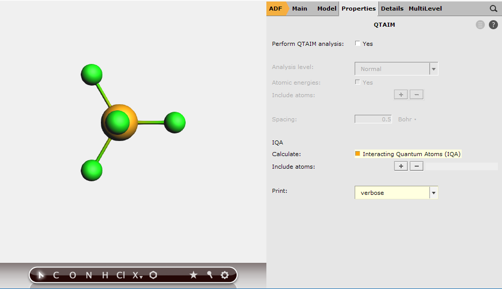
Step 4: Build PF₅, optimize and calculate all interactions¶

We will now look at the P-F bonds in the PF₅ molecule.

Note that you can combine the geometry optimization with an IQA calculation, which we will now do for PF₅.

Close all previous windows and start again AMSinput.
Build a trigonal bipyramidal structure:  Structure Tool → Metal Complexes →  ML5 trigonal bipyramidal.
Change the central atom into a P atom.
Change ligands into F atoms.
Choose the Geometry Optimization task in main section.
Set Relativity: None, Basis set: DZP, and Frozen core: None.

In the panel bar, select Properties → QTAIM.
Check the Calculate: Interacting Quantum Atoms (IQA) check-box.
Set Print to verbose.
Save and Run.

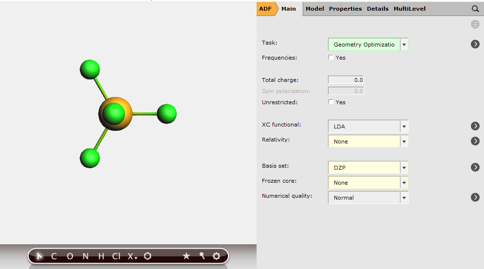
At the end of the calculation, AMSinput will ask whether to use the new coordinates. Select No.

Step 5: Analyze the results and compare equatorial and axial P-F bonds¶

When the calculation has finished, check the results:

Open the output file: SCM → Output

Search for the IQA section

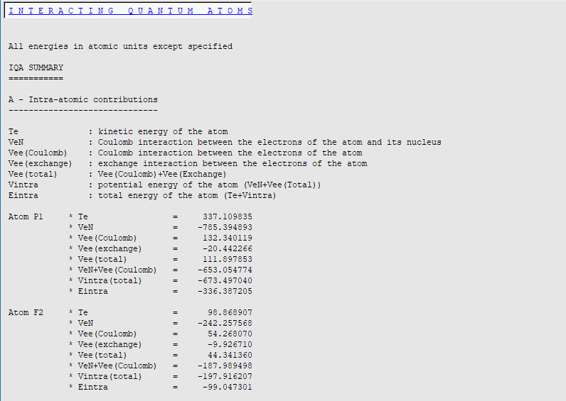
In this verbose mode, more information is printed: individual terms for intra- and inter-atomic interactions are printed and a total energies section is added.

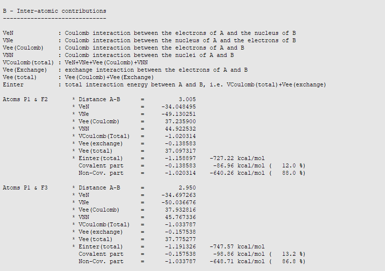
The bonds with equatorial fluorine atoms can be recognized by the interatomic distance of 2.95. These bonds are predominantly ionic (87-88%) with interaction energies between -748 and -760 kcal/mol (-756 kcal/mol on average). The difference between equatorial bonds can be explained by the fact that the assignment of the integration points located near the border between two QTAIM basins is somewhat arbitrary. The different can be reduced by increasing the numerical quality to Good and VeryGood. Please note that this inter-atomic energy should not be confused with a bond formation energy that includes the variations of intra-atomic terms during the bond formation and substantial secondary interactions between the incoming fluorine atom and other fluorine atoms.

The axial P-F bonds are longer than the equatorial ones. Therefore, we may expect them to be weaker and the IQA energy decomposition analysis confirms our chemical intuition. Indeed, the covalent contribution to the interaction decreases (from about -97 kcal/mol to -87 kcal/mol) and so does the classical Coulomb interaction (from -650 kcal/mol to -640 kcal/mol). This results in a substantial decrease of the total inter-atomic interaction from -756 kcal/mol to -727 kcal/mol, in agreement with the bond length increase.

Regarding accuracy of the results, classical Coulomb interaction energies (Non-Cov. part) can be extremely sensitive to the choice of the basis set. This can be seen in the following table (geometry optimized at the LDA/DZP level; normal numerical quality):

XC/Basis           P-F(eq) min      P-F(eq) max         P-F(ax)
PBE0/DZP           -730             -743                -713
PBE0/TZP           -728             -769                -735
PBE0/TZ2P          -786             -816                -773
PBE0/QZ4P          -793             -796                -774

The quality of the integration grid is also important for evaluating the electrostatic (Non-Cov. part) contribution. We recommend the numerical quality VeryGood when accurate energies are required. The Normal level can be used for semi-quantitative purposes. This can be seen in the following table obtained at the PBE0/DZP level (for a geometry optimized at the LDA/DZP level and a normal numerical quality):

Quality           P-F(eq) min      P-F(eq) max         P-F(ax)
Basic             -687             -766                -700
Normal            -731             -743                -714
Good              -719             -728                -697
VeryGood          -723             -725                -718

It’s noteworthy that the asymmetry between equatorial atoms (P-F(eq) min and max) becomes rather small at the numerical quality VeryGood.