Eu3+ Luminescence properties with Ligand Field DFT
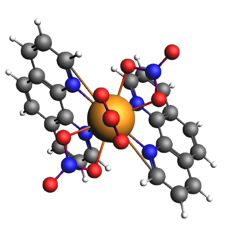
Eu3+ compounds are often used in trichromatic phosphors for lighting purposes, where they are known for red-color emission. The red emission results from the Eu 4f6 → 4f6 transitions involving the ground states 7FJ (with J designating the spin-orbit components, i.e., 0, 1, 2, … , 6), and low-lying excited state 5D0. In this tutorial, we are going to calculate the energy levels of Eu3+ compounds by using LFDFT, in order to understand the mechanism of the electron transition process. As example for application, we consider the luminescence properties of the compound [Eu(NO3)3(phenanthroline)2]. More detailed calculation procedure can be found in Ref. [1].
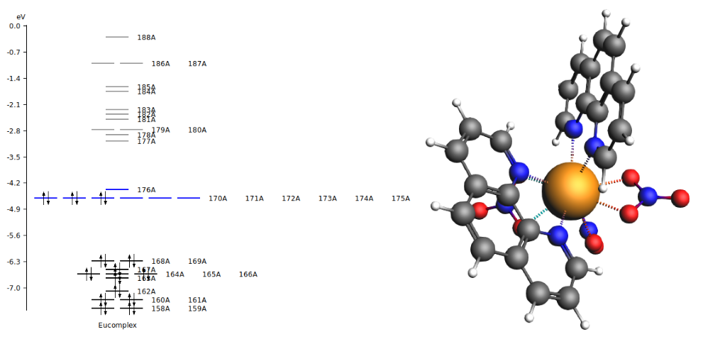
[Eu(NO3)3(phenanthroline)2] has an open-shell electronic structure, where the Eu 4f orbitals are occupied with 6 valence electrons. In accord with the LFDFT method we have to define an average of configuration type calculation. We use the keyword “IRREPOCCUPATIONS” in ADF to set fractional electron occupations of the molecular orbitals. For [Eu(NO3)3(phenanthroline)2], 338 electrons are restricted to closed shell, and 6 valence electrons are evenly distributed over the seven molecular orbitals that are identified with large atomic 4f characters and thus constitute the active subspace of the ligand-field calculation.
LFDFT atomic database installation
To run LFDFT you need to first install the LFDFT atomic database on the machine where you run the calculation.
Setting up the calculation
We start by downloading the input structure Eu-complex.xyz, a file that contains the cartesian
coordinates of the Eu3+ complex [Eu(NO3)3(phenanthroline)2].
Remark: the first atom in a LFDFT calculation needs to be the atom of interest, Eu in this case.
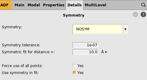
Before the actual Ligand Field DFT calculation (LF-DFT), a preliminary DFT calculation is run. From this calculation the occupation numbers of the molecular orbitals are obtained. The occupation numbers are then used to set up the LF-DFT calculation. This can be a cheap calculation, as long as the basis set is all electron and the symmetry is NOSYM. There is no need for a converged SCF.

1 for ‘Maximum number of SCF cycles’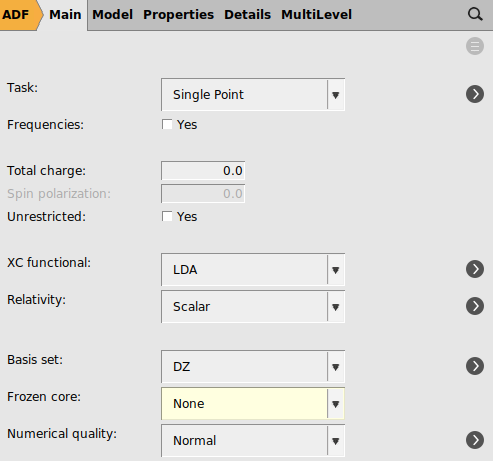
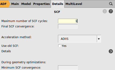
The calculation will not converge (because of the difficult open-shell electronic structure and 1 SCF cycle), but the output can be used to set fractional occupations to the molecular orbitals later. Once the calculation is finished, click OK to the error message that the SCF did not converge.
Important is to change the number of SCF cycles back to the original value.
300 for ‘Maximum number of SCF cycles’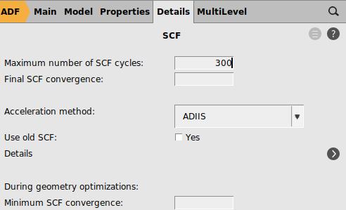
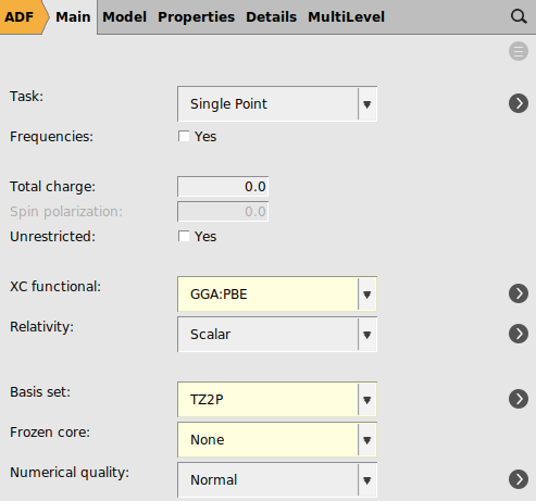
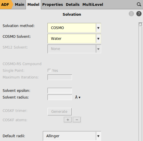
Next we will try to use the settings as were used in Ref. [1] for PBE. The calculation is performed in water using COSMO as solvation method.
LFDFT requires an average of configuration (AOC) run. The occupation numbers will reflect an AOC where 338 (= 169*2) electrons are in doubly occupied orbitals, and 6 valence electrons are evenly distributed over the 7 molecular orbitals that are identified with large atomic 4f characters.
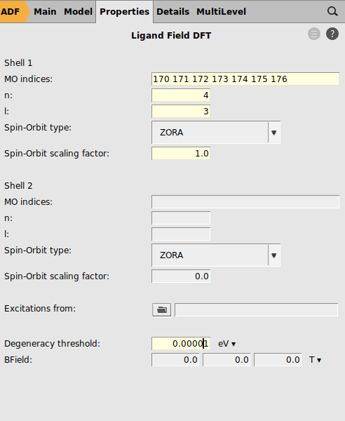
The MO indices in the LFDFT settings should be the fractionally occupied levels of the AOC calculation. In the LFDFT run spin-orbit coupling will be included. In the results we want to see all spin-orbit splitted levels even if they are close. Therefore a small degeneracy threshold is chosen.
6/7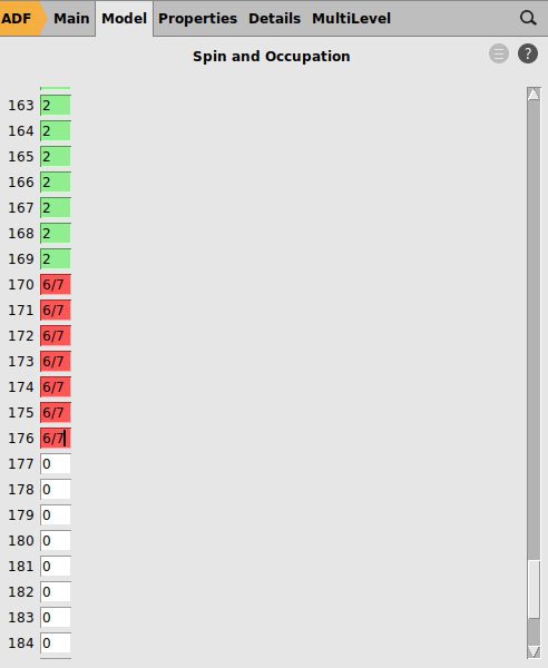
Results
Once the calculation is finished (may take several minutes), the molecular orbitals and the occupation numbers of the 4f orbitals can be found in the output file.
 → Output
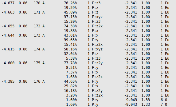
Scroll down to molecular orbitals #170, 171, …, 176 to verify that they have predominantly Eu f character and are occupied with fractional 6/7 = 0.86 electrons.
→ SpectraBelow the figure in AMSspectra a list of all the calculated energy levels is given. This includes all levels of the Eu 4f6 configuration split by spin-orbit coupling and ligand field, in total 3003 values.
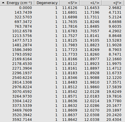
The lowest 49 levels all have expectation values of <S2> close to 12 and <L2> close to 12, which means a high 7F character.
Similarly, if one scrolls down one can find that levels 50-58 have high 5D character.
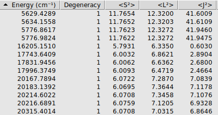
The calculated levels can be compared to the calculated ones for PBE in the paper. The lowest 7F levels in cm-1 are 0, 144, 323, 698, versus 0, 214, 393, 700 for PBE in the paper, and the lowest 5D levels are at 16205, 17744, 17832, 17996 versus 16081, 17705, 17716, 17806 for PBE in the paper. The agreement is reasonable, however, apparently small differences in the calculation can lead to somewhat larger differences in the energy of the levels, and can easily lead to a difference of a few 100 cm-1.
In the output one can find a more detailed spectral analysis of the results.
→ Output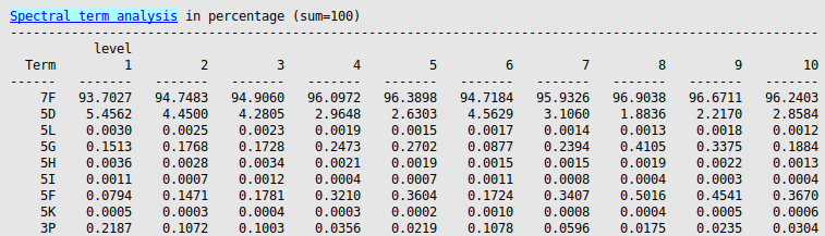
In this results block, the energy levels are projected on to the atomic solution, giving rise to the listed percentage characters.
Instead of PBE one can also use, for example, the hybrid PBE0, and use the same settings as before.
This, however, will take much more time (may take several tens of minutes). One could skip this part and only look at the results. Note again that small differences in the calculation can lead to somewhat larger differences in the energy of the levels.
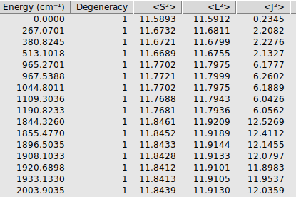
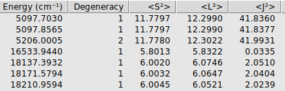
Again the lowest 49 levels have a high 7F character and levels 50-58 have high 5D character. Now labeling the levels with a J value makes more sense than in the PBE calculation. The lowest level has an expectation values of <J2> close to 0 thus this level could be labeled as 7F0, levels 2-4 have an expectation values of <J2> close to 2 thus this level could be labeled as 7F1, etcetera.
The table compares a subset of LFDFT/PBE0 energy levels with the experimental values reported in Ref. [1].
State |
PBE0 (cm -1) |
Exp (cm -1) |
|---|---|---|
7F0 |
0 |
0 |
7F1 |
267 |
295 |
380 |
367 |
|
513 |
444 |
|
7F2 |
965 |
947 |
968 |
981 |
|
1045 |
1016 |
|
1109 |
1080 |
|
1190 |
1111 |
|
… |
||
5D0 |
16534 |
17241 |
5D1 |
18137 |
18945 |
18172 |
||
18211 |