L-Edge X-Ray spectrum NEXAFS
XANES or NEXAFS is a process where core electrons are excited by X-ray photons. Knowing the X-ray spectrum can help in determining the electronic structure of the atoms in a molecule. In this tutorial we will calculate the excitations of a Si 2p core electron of SiCl4 using the ADF engine. X2C spin-orbit coupled relativistic calculations will be performed. Compared to ZORA the relativistic methods X2C and RA-X2C give a better description of core orbitals. First the transition potential method (TP) will be used and next TD-DFT.
The cheap TP method is useful especially for K-Edge X-ray spectra, but also for L-Edge it will give a reasonable spectrum, however, the relative intensities for the spin-orbit splitted levels of the 2p are typically not so great. With the more expensive TD-DFT method one can improve these relative intensities for L-Edge 2p electrons.
Note
This tutorial is also available in video format.
Step 1: Setting up the system
SiCl4.xyz and import them into AMSinput (the system should have
 T(D) symmetry)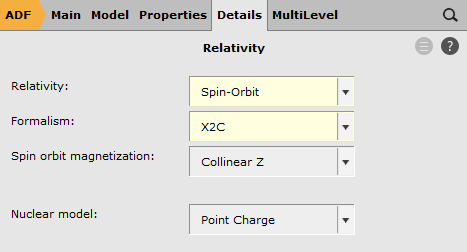
 button to create a new region and call it
 SR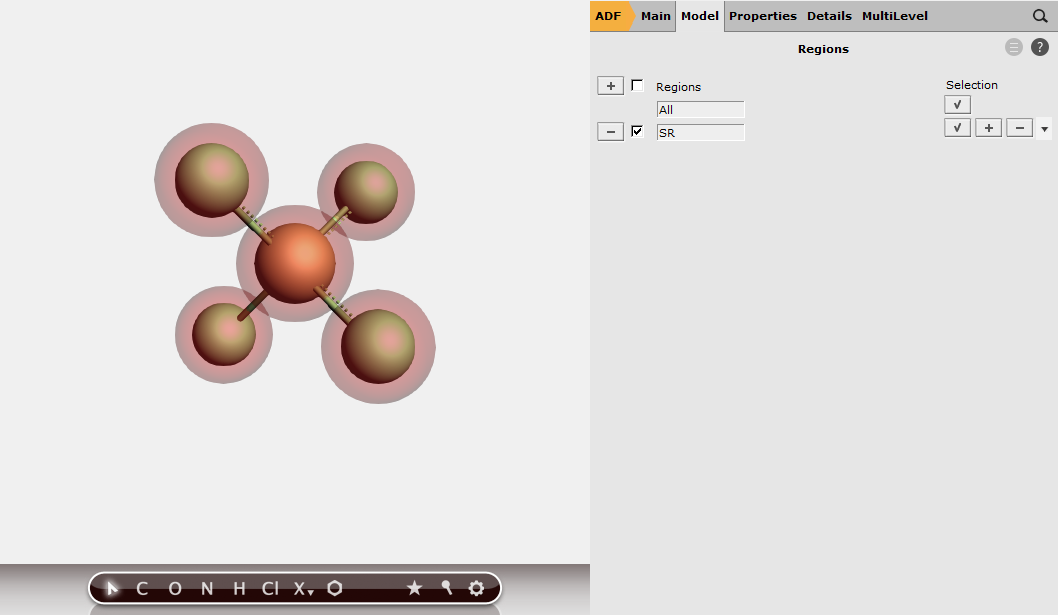
SO and run itStep 2: Selecting the orbital labels
In order to excite a 2p electron we need to know the orbital labels first.
The diagram should look like this:
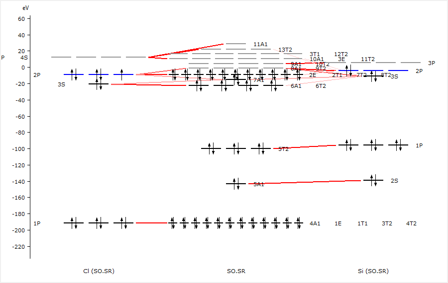
The Si 2p orbitals are labeled as 1P and form the 5T2 labeled orbitals in SiCl4 and have energies of around -100 eV. We performed spin-orbit relativistic calculations which will have split these orbitals and changed their labels.
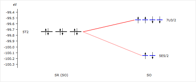
We see that the 5T2 orbitals have been split into 7U3/2 and 5E5/2 spinors. We will use these labels now to excite a 2p electron.
Step 3: TP method
The TP method is fast and one can easily afford a large basis set. The TP method is approximate and using LDA will not make the approximation much worse. One should not use the TP method with a hybrid functional. In the TP method 0.5 electron will be removed, in this case 0.5 electron from the (almost) degenerate Si 2p orbitals (spinors).
SO.results/adf.rkf5E5/2 to 11/67U3/2 to 11/3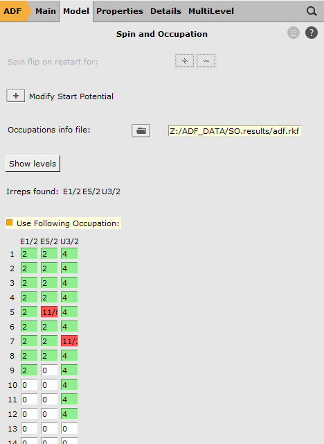
40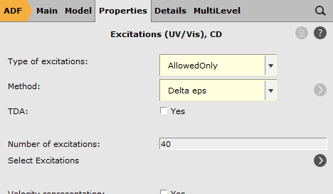
7U3/2 5E5/2 as ‘Occupied orbitals’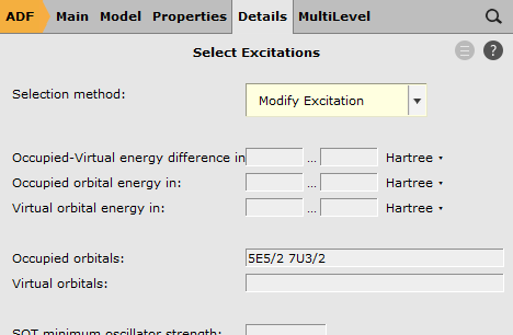
Here we have selected the orbitals to excite from. We have removed, in total, 1/2 electron from the Si 2p orbitals. These Si 2p orbitals (in the scalar relativistic calculation these are the 5T2 orbitals) were split into a four-fold degenerate 7U3/2 spinor and a two-fold degenerate 5E5/2 spinor. Therefore we have removed 1/6 electron from 5E5/2 and 1/3 electron from 7U3/2.
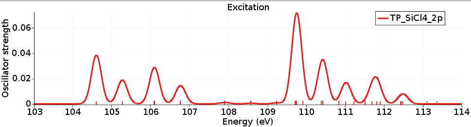
The X-ray spectrum can be seen with SCM → Spectra (Horizontal unit eV, and Width 0.3) and shows the L-edge of the SiCl4 molecule. It can be compared against experimental spectra (for example, R. Püttner, M. Domke, and G. Kaindl, Phys. Rev. A 57, 297 (1998)).
The calculated excitation energies are in reasonable agreement, however, the relative intensities (of the first 4 peaks) are not so great.
The difference in energy between the lowest two peaks is due to the spin-orbit splitting of the Si 2p orbital, which is calculated to be a bit more than 0.6 eV.
Step 4: TD-DFT
The TP method that was used in the previous step is fast and gives a reasonable spectrum if one compares it to experiment, but for L-edge 2p the calculated relative intensities (of the first 4 peaks) are not so great. The intensities can be improved for L-edge 2p if TD-DFT is used. Here the SAOP model potential is used, since it is also good for Rydberg states and is relatively cheap to calculate. Note, however, that TD-DFT is much slower than the TP method. Make sure to open a new AMSinput window.
407U3/2 5E5/2 as ‘Occupied orbitals’TDDFT_SiCl4_2p and run the calculation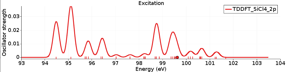
Again the X-ray spectrum can be seen with SCM → Spectra (Horizontal unit eV, and Width 0.3) and shows the L-edge of the SiCl4 molecule. It can be compared against experimental spectra (for example, R. Püttner, M. Domke, and G. Kaindl, Phys. Rev. A 57, 297 (1998)).
The calculated excitation energies are shifted compared to experiment with about 10 eV, and are thus in worse agreement than the results with the TP method.
However, the relative intensities (of the first 4 peaks) are improved with respect to the results with the TP method.
It is not uncommon to shift the calculated spectrum in such cases. It depends on the XC functional and to a lesser extent on the basis set how large this shift is. If results for excitations of a certain orbital of a given element are compared for different molecules one typically uses the same shift in energy. Compared to SAOP the much more expensive TD-DFT calculations with a hybrid functional with approximately 50% HF exchange seem to give improved excitation energies, if these are compared to experiment. Note that also the very cheap TP method seem to be capable of doing that.