Charge Displacement¶

The Charge-Displacement (CD) analysis is a simple method able of analyzing and quantifying the amount of charge transfer that occurs upon a bond formation between two interacting fragments. This tutorial shows three different examples how to calculate the Charge-Displacement function.

The CD function Δq(z) is defined as the partial integration along a chosen axis, z, of the electron density rearrangement Δρ(x,y,z’) taking place upon the bond formation:

\[\Delta q(z) = \int_{-\infty}^\infty dx \int_{-\infty}^\infty dy \int_{-\infty}^z dz' \Delta \rho (x,y,z')\]

It can be also used in combination with the NOCV theory (where the electron density rearrangement is defined with respect to the orthonormalized non-interacting fragments). More information about Natural Orbitals for Chemical Valence can be found at ETS-NOCV and in the EDA-NOCV tutorial. In this case the deformation density can be expressed as a sum of contributions (Δρ_k) defined by the NOCV pairs of complementary eigenfunctions (Ψ_-k and Ψ_k) corresponding to eigenvalues -ν_-k and ν_k with the same absolute value but opposite sign:

\[\Delta \rho_k(z) = v_k ( -| \Psi _{-k}|^2 + | \Psi _{+k}|^2 )\]

and the associated CD function (NOCV-CD) is simply defined as following:

\[\Delta q_k(z) = \int_{-\infty}^\infty dx \int_{-\infty}^\infty dy \int_{-\infty}^z dz' \Delta \rho_k (x,y,z')\]

This tutorial shows how to build the chemical integrands for evaluating the CD function in three different relevant examples:

Quantifying the CT contribution in closed-shell interacting fragments: case of noble metal-noble gas interaction in the Xe-AuF complex. [1]
Quantifying of the Dewar-Chatt-Duncanson bonding components (σ-donation and π-backdonation) in transition metal complex applying the CD function in combination of the NOCV theory (NOCV-CD). [2]
Application to open-shell systems to reveal competing pathways of proton-coupled electron transfer in oxidation catalysis (hydrogen-atom transfer, concerted proton-coupled electron transfer). [3]

In all cases the basic idea is to evaluate the different integrands (Δρ, Δρ_k or Δρ_α/β) using densf or directly from AMS-GUI which allow for their efficient mapping of a grid (CUBE format).

The CD function is evaluated numerically on the grid. This tutorial will make use of auxilary programs distributed with AMS. We will give all the details and scripts for using the PYCUBESCD suite of programs which is freely available (LGPL-3.0 License at GitHub).

Case 1: CT in closed-shell interacting fragments: Xe—AuF¶

The molecular structures needed for this tutorial are given here. The molecular structures are properly aligned with the molecular axis along the z axis. In general, one should optimize the structures first and align with the z axis coinciding with the direction chosen for evaluating the CD function.

Note

The alignment is important. The z axis defines the axis on which is performed the partial integration for evaluating the CD function. The fragments (Xe and AuF) have the geometry they possess within the complex.

1. Fragment Calculation¶

At first, a fragment calculation must be performed. The following steps from the Fragment Analysis tutorial can be followed. Alternatively this frag_XeAuF.run script can be runned. A script including the fragment calculation (step 1) and step 2 will be provided in step 2.

: Start AMSinput and insert the Xe-AuF structure.

In the Main ADF Panel, select the Single Point task

Select the GGA:BLYP XC functional

Make sure the Relativity is set at Scalar

Select a TZ2P Basis set, a Small Frozen core

Select a Good Numerical quality

In the Panel bar, select Model → Regions

Select Xe and click the to add it as region

Select the Au and F and add them as a second region

In the Panel bar, select MultiLevel → Fragments

Check the Use fragment box

Save and run the calculation

The .rkf file of the final fragment analysis (the adf.rkf in the XeAuF.results folder) is needed in the following step.

2. Density SCF¶

The densf program must be used, which is an auxiliary program distributed with ADF suite. See the documentation of Densf: Volume Maps to generate a numerical representation of the electron densities associated with the XeAuF complex and the sum of the isolated Xe and AuF fragments. Herein, details for the definition of the grid can be found. We will map these quantities in the CUBE format. The only information necessary from the previous fragment calculation (Step 1) is the rkf file.

The following script can be used to generate a CUBE file using densf for the SCF electron density (Density SCF):

"$AMSBIN"/densf << eor
INPUTFILE FragmentCalcXeAuF.rkf      ! This is the rkf file used as input
Density SCF                          ! We require the SCF density to be mapped
CUBOUTPUT XeAuF                      ! We specify a name (option)
grid                                 ! Definition of the grid
 -10.0 -10.0 -10.0
 100  100  100
 1.0 0.0 0.0 15.03
 0.0 1.0 0.0 15.03
 0.0 0.0 1.0 15.03
end
end input
eor

A CUBE file can also be generated using densf for the sum of the SCF electron densities of the isolated Xe and AuF fragments (Density SumFrag):

"$AMSBIN"/densf << eor
INPUTFILE FragmentCalcXeAuF.rkf      ! This is the rkf file used as input
CUBINPUT
Density SumFrag                      ! We require the Sum of SCF densities of the isolated Fragments
CUBOUTPUT XeAuF                      ! We can specifies a name
grid                                 ! Definition of the grid
-10.0 -10.0 -10.0
100  100  100
1.0 0.0 0.0 15.03
0.0 1.0 0.0 15.03
0.0 0.0 1.0 15.03
end
end input                            ! Output is the file: XeAuF%SumFrag%Density.cub
eor

A script to generate the two cubes for XeAuF and the sum of the electron densities of the Xe and AuF can also be downloaded here.

Note

All densities must be mapped on the same numerical grid. This has been explicitly defined after the grid keyword in the densf input. This is important if you use the PYCUBESCD suite of programs to calculate the CD function in Step 3.

3. Generate CD function¶

Now we use the PYCUBESCD suite of programs to make operations between Cube files and to generate the CD function. PYCUBESCD suite is freely available to download (LGPL-3.0 License at GitHub) and can be used both with python2 and python3 (it requires only Numpy as extra module).

In the following command, $INSTALL is the directory where the PYCUBESCD program is installed. You make use of the pysub_cube.py file which is placed in the PY3 folder in the pycubescd-master.

Run the following command in order to generate the file diff_XeAuF.cub, which contains the numerical representation of the electron density difference between the XeAuF molecule (cube file: XeAuF%SCF%Density.cub) and the sum of the electron density of the Xe and AuF fragments (cube file: XeAuF%SumFrag%Density.cub) obtained in the Step 2:

python3 $INSTALL/PY3/pysub_cube.py -f1 XeAuF%SCF%Density.cub -f2 XeAuF%SumFrag%Density.cub -o  diff_XeAuF.cub

This file (diff_XeAuF.cub) can be easily visualized within AMS-GUI:

: Open → View

Open the diff_XeAuF.cub file (File → Open…)

Add → Isosurface: With Phase

Select the field generated

Change the isovalue to 0.0005 e/au³

The CD function can be generated by using the pycd_simple.py program available in PYCUBESCD suite ($INSTALL is the directory where the PYCUBESCD program is installed):

python3 $INSTALL/PY3/pycd_simple.py -f diff_XeAuF.cub

The result is a text format file (diff_XeAuf.cub_cdz.txt) which contains the numerical representation of the CD function. It can be easily visualized with a 2D-plot software.

Case 2: Dewar-Chatt-Duncanson bonding components in a transition metal complex (NOCV-CD)¶

This tutorial shows how to generate the NOCV deformation densities (Δρ_k) and export them on a numerical grid (CUBE file format) directly using AMS-GUI. The associated CD functions (Δq_k) are evaluated numerically using the PYCUBESCD suite of programs, freely available at GitHub.

The transition state complex needed for this tutorial is given here.

Note

The alignment of the molecule is important. The z axis defines the axis on which is performed the partial integration for evaluating the CD function. In this case the integration axis is defined as the axis passing for the Ni atom and the midpoint of the CC triple bond of the coordinated alkyne.

1. Fragment Calculation¶

: Start AMSinput and insert the transition state complex

In the Main ADF Panel, select the Single Point task

Select the GGA:BLYP XC functional

Make sure the Relativity is set at Scalar

Select a TZ2P Basis set and a Good Numerical quality

In the Panel bar, select Model → Regions

Select the C₂ H₂ and click the to add it as region

In the menu bar, click Select → Invert Selection and add them as a second region

In the Panel bar, select MultiLevel → Fragments

Check the Use fragment box

In the Panel bar, select Properties → ETS-NOCV

Select the Closed-Shell at ETS-NOCV analysis

Save and run the calculation

2. Visualize NOCV deformation densities¶

The NOCV deformation densities can be visualized by performing the following steps:

: Open → View of the Fragment Calculation

In the menu bar, select Add → Isosurface: With Phase

Select Field … → NOCV Def Densities

Select a deformation density, for instance Δρ₁

Change the isovalue to 0.003 e/au³

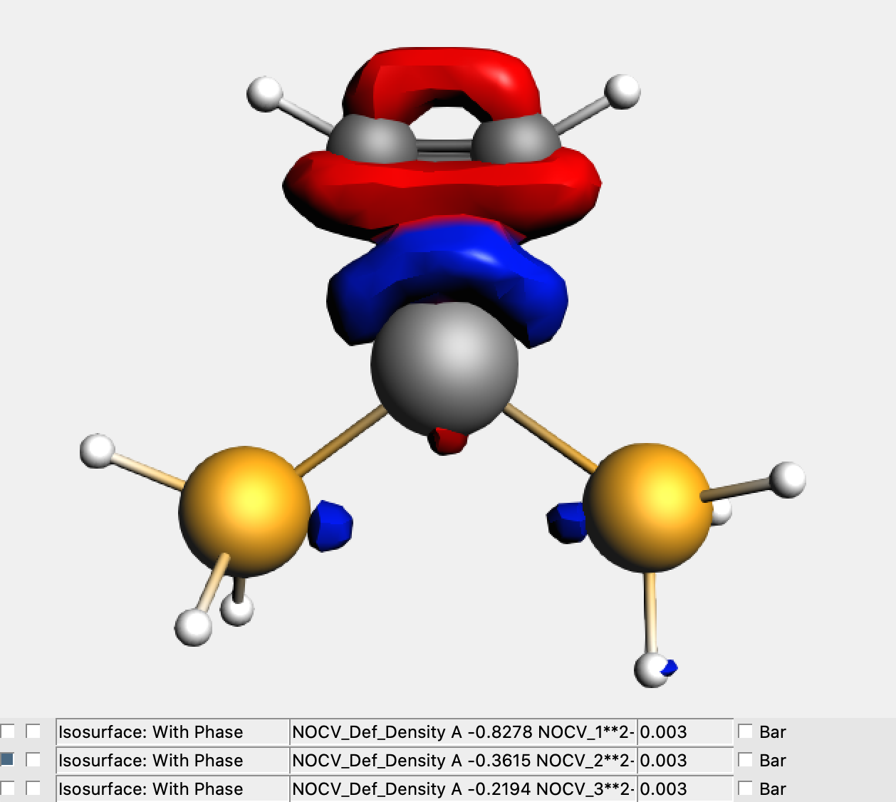
In the above figure is shown the deformation density (Δρ₁) associated with the largest NOCV eigenvalue. It clearly represents the metal-to-substrate π-backdonation (red/blue colored isodensity surface defines electron density depletion/accumulation).

3. Generate a CUBE file¶

One starts with adding all the NOCV deformation densities you want to map in Cube File format. For instance, in the below example we chose those associated with the three largest eigenvalues, namely 0.8278, 0.3615 and 0.2194. The isodensity surface in the figure is related to Δρ₂, which is clearly related to the σ-substrate-to-metal donation component. You add the NOCV deformation densities with:

: Add → Isosurface: With Phase

Select Field … → NOCV Def Densities

The CUBE file can be generated now:

: Improve the Course Gris by selecting Fields → Grid → Medium (or Fine)

In the menu bar, select File → Export Field as Cube Files

Note

Typically the Medium setting for the Grid is sufficient to obtain accurate CD functions. Clearly, the larger the grid is, the larger the size of the generated Cube files will be. For instance using Medium Grid the three Cube Files associated at Δρ₁,Δρ₂,Δρ₃ have a size of 4.3MB (the latter increases to 34.3MB whether one sets Fine Grid to generate Cube Files).

4. CD functions for the NOCV deformation densities¶

The CD functions are generated using the pycd_simple.py program available in PYCUBESCD suite (exactly as done in the Case 1, step 3):

Give the following command line in the directory where the Cube Files associated at Δρ₁, Δρ₂, and Δρ₃ have been generated (in the .results folder) and in which $INSTALL is the directory where the PYCUBESCD program is installed:

python3 $INSTALL/PY3/pycd_simple.py   -f  215--Medium-0.cube%NOCV%SumDensities_A_1.cub

python3 $INSTALL/PY3/pycd_simple.py   -f  218--Medium-0.cube%NOCV%SumDensities_A_2.cub

python3 $INSTALL/PY3/pycd_simple.py   -f  221--Medium-0.cube%NOCV%SumDensities_A_3.cub

The results are three text format files (.cub_cdz.txt) which contains the numerical representation of the CD functions associated with Δρ₁, Δρ₂, and Δρ₃. They can be easily visualized with a 2D-plot software. The picture below can be obtained combining the 3D isosurface pictures of the NOCV density deformations.

Case 3: Open-Shell CD in the HAT mechanism of the TauD-J intermediate¶

This tutorial shows how to generate the spin-density difference and the total-density difference (Δρ_α,Δρ_β,Δρ_tot) and export them on a numerical grid (CUBE file format) using densf. The associated CD functions (Δq_α,Δq_β,Δq_tot) are then evaluated numerically using the PYCUBESCD suite of programs, freely available at GitHub.

1. Unrestricted Calculations¶

First, we need to perform a set of unrestricted ADF calculations on the transition state structure of the TauD-J__C₂ H₆ model system. The TauD-J intermediate features a Fe^IV =O unit which is the H-abstracting species. The two consituting fragments to consider are the Fe=O moiety of TauD-J and the C₂ H₆ substrate, in the position they occupy in the transition state geometry. The molecular structures needed for this tutorial can be downloaded here.

Note

The alignment of the molecule is important. The z axis defines the axis on which is performed the partial integration for evaluating the CD function. In this case the integration axis is defined as the axis thrrough the Fe=O bond.

Three indipendent calculations will be performed: (i) TauD-J__C₂ H₆ model system (FeO_CH) (ii) TauD-J fragment (FeO) and (iii) ethane fragment.

: 1. Start AMSinput and insert the TauD-J__C2H6 system

2. In the Main ADF Panel, select the Single Point task

3. Tick the Unrestricted calculation box

4. Fill in for the Spin polarization 4.0

5. Select the GGA-D:S12g-D3 XC functional

6. Make sure the Relativity is set at Scalar

7. Select a TZ2P Basis set, a Small Frozen core

8. Select a Good Numerical quality

9. Save and run the calculation

Now, the other two single point calculations can be performed:

: Insert the TauD-J fragment in a new AMSinput

Repeat step 2-9 from above

: Insert the ethane fragment in a new AMSinput

Select the Single Point task

Tick the Unrestricted calculation box (Spin polarization of 0.0)

Repeat step 5-9 from above

The adf.rkf files of these calculations are needed for the following step.

2. Generate CUBE files¶

We use densf to generate a numerical representation of the electron spin-densities associated with the unrestricted calculations performed on the (i) TauD-J__C₂ H₆ model system (FeO_CH) (ii) TauD-J fragment (FeO) and (iii) ethane fragment (CH). We map these quantities in the CUBE format. The only information necessary from previous single point calculations are the adf.rkf files (here renamed as FeO.rkf, CH.rkf and FeO_CH.rkf).

The following script can be used to generate a CUBE file:

$ASMBIN/densf << eor
ADFFILE FeO.rkf             ! this is the rkf file used as input
Density SCF                 ! We require the SCF density to be mapped
CUBOUTPUT FeO               ! We specify a name (option)
grid                        ! Definition of the grid (for details, see tutorial Densf: Volume Maps)
 -10.0 -10.0 -10.0
 300  300  350
 1.0 0.0 0.0 20.0
 0.0 1.0 0.0 20.0
 0.0 0.0 1.0 20.0
end
end input
eor

Note

As in any unrestricted calculation, we will get the α- and β-spin electron density as a result.

Similarly, the CUBE files for the SCF electron spin-density of the C₂ H₆ fragment and the TauD-J__C₂ H₆ model system can be generated. We will obtain the α- and β-spin electron densities of FeO, CH and FeO_CH as a result.

3. Obtain density differences¶

We now use the PYCUBESCD suite of programs to make operations between Cube files and to obtain the spin-density differences (Δρ_α, Δρ_β) and the total density difference (Δρ). These density differences will be then integrated along the z axis to retrieve the corresponding CD functions.

Use the command lines below in the directory where your just generated cube files are placed. The $INSTALL need to be changed to the directory where the PYCUBESCD program is installed, and when you have named the cuboutput differently (than FeO, CH and FeO_CH) change the names of the input cube files as well.

python3 $INSTALL/PY3/pyadd_cube.py -f1 FeO%SCF%Density_A.cub -f2 CH%SCF%Density_A.cub -o  SumFrag_Density_A.cub

python3 $INSTALL/PY3/pyadd_cube.py -f1 FeO%SCF%Density_B.cub -f2 CH%SCF%Density_B.cub -o  SumFrag_Density_B.cub

python3 $INSTALL/PY3/pysub_cube.py -f1 FeO_CH%SCF%Density_A.cub -f2 SumFrag_Density_A.cub -o  diff_FeO_CH_A.cub

python3 $INSTALL/PY3/pysub_cube.py -f1 FeO_CH%SCF%Density_B.cub -f2 SumFrag_Density_B.cub -o  diff_FeO_CH_B.cub

python3 $INSTALL/PY3/pyadd_cube.py -f1 diff_FeO_CH_A.cub -f2 diff_FeO_CH_B.cub -o diff_FeO_CH.cub

The generated diff_FeO_CH_A.cub, diff_FeO_CH_B.cub and diff_FeO_CH.cub files contain the numerical representation of the electron (spin) density difference between the FeO_CH system and the sum of the electron (spin) densities of the FeO and CH fragments.

These files can be easily visualized within AMS-GUI in the same manner as for Case1 and Case2:

: Open → View

Open a diff_FeO_CH.cub file (File → Open…)

Add → Isosurface: With Phase

Select the field generated

Change the isovalue to 0.01 e/au³

4: Generate the CD functions¶

The CD functions are finally generated using the pycd_simple.py program available in PYCUBESCD suite. Again, the $INSTALL needs to be changed to the directory where the PYCUBESCD program is installed.

python3  $INSTALL/PY3/pycd_simple.py -f diff_FeO_CH_A.cub

python3  $INSTALL/PY3/pycd_simple.py -f diff_FeO_CH_B.cub

python3  $INSTALL/PY3/pycd_simple.py -f diff_FeO_CH.cub

This results in three text formal files ( .cub_cdz.txt) which contains the numerical representation of the CD functions associated with Δρ_α, Δρ_β and Δρ_tot. They can be easily visualized with a 2D-plot software. The picture below can be obtained combining the iosurface picture of the total density difference and the three CD functions.

References¶

[1]	Belpassi, I. Infante, F. Tarantelli, L. Visscher, The Chemical Bond between Au(I) and the Noble Gases. Comparative Study of NgAuF and NgAu+ (Ng = Ar, Kr, Xe) by Density Functional and Coupled Cluster Methods, Journal of the American Chemical Society 130, 1048 (2008).

[2]	Bistoni, S. Rampino, F. Tarantelli, L. Belpassi, Charge-displacement analysis via natural orbitals for chemical valence: Charge transfer effects in coordination chemistry, Journal of Chemical Physics 142, 084112 (2015).

[3]	D’Amore, L. Belpassi, J. E. M. N. Klein, M. Swart, Spin-resolved charge displacement analysis as an intuitive tool for the evaluation of cPCET and HAT scenarios Chemical Communications 56, 12146 (2020).