Mode Refinement

In this tutorial we use the Mode Refinement method to calculate the high energy end of the IR spectrum of the dydrogesterone molecule. In order to reduce the computational time of this tutorial we are using DFTB as the target method and UFF as the approximate method providing the basis in which to express the DFTB modes. In reality one would rather use DFTB as the approximate method and refine the modes at the DFT level.

More information on these features can be found in the AMS user manual:

• Vibrational spectroscopy section of the AMS manual
• Mode Refinement section of the AMS manual

Let us first calculate the entire IR spectrum of dydrogesterone at the DFTB level. This is our reference spectrum which we will later try to reproduce using the Mode Refinement method. Since DFTB is a fast engine, calculating the entire spectrum does not take a long time.

1. Start AMSjobs.

2. Click on SCM → New Input. This will open AMSinput.

3. In AMSinput, insert the dydrogesterone molecule by clicking the search icon and typing “dydrogesterone” into the box. Select the “C21H28O2: Prodel” entry from the molecules section.

4. Select the DFTB panel: →

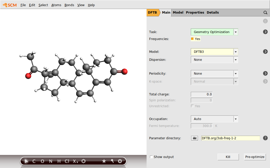
5. In order to calculate the full IR spectrum, make sure Task is set to Geometry Optimization and tick the Frequencies checkbox.

6. Select Model → DFTB3, and Parameter directory → DFTB.org/3ob-freq-1-2.

Your AMSinput window should look like this:

We are now ready to run the calculation:

1. Click on File → Save As… and give it the name “DFTB_GOFREQ”.

2. Click on File → Run . This will bring the AMSjobs window to the front.

3. Wait for the calculation to finish …

4. When AMSinput asks if it should update the geometry to the optimized geometry, select Yes.

We now have optimized the geometry of dydrogesterone at the DFTB3 level of theory, and calculated its IR absorption spectrum. Let us look at the spectrum we obtained.

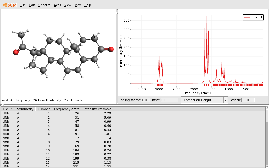
1. Click on SCM → Spectra. This will show the IR spectrum of dydrogesterone in AMSspectra.

You should see the following IR spectrum (to obtain the same graph, make sure to set the peak width to 11):

A useful tool for understanding the IR spectrum is the Partial Vibrational Spectra (PVDOS) analysis.

1. In AMSspectra click on Spectra → Partial Vibrational Spectra (PVDOS)

2. Select, for example, all atoms with a double bond

You will see that the normal modes involving C=C and C=O bonds atoms are mostly located at around 1600cm^-1.

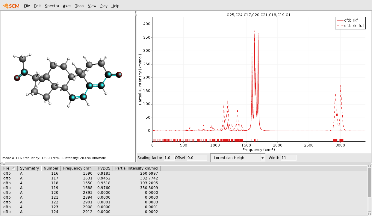
By clicking the individual peaks in the spectrum you can see the corresponding mode in the viewpoint on the left. Looking at the spectrum and the contained modes one can see that:

1. The spectral region around 3000cm^-1 contains all modes with C-H stretch character. There are 28 modes in this window, since there are 28 C-H bonds in the system.
2. Around 1600cm^-1 we have 4 IR intense modes involving the stretching of the C=C and C=O bonds.
3. The other 115 modes below 1500cm^-1 feature all kinds of collective bending modes involving large parts of the entire molecule.

We will now attempt to reproduce the first two bands mentioned above, that is the C-H stretch and C=C/C=O stretch bands, using Mode Refinement, i.e. without calculating the entire spectrum at the DFTB level.

In order to use Mode Refinement, we first need a basis of approximate normal modes. These are typically normal modes obtained at a lower (and therefore faster) level of theory. Here we will use UFF to calculate these approximate modes.

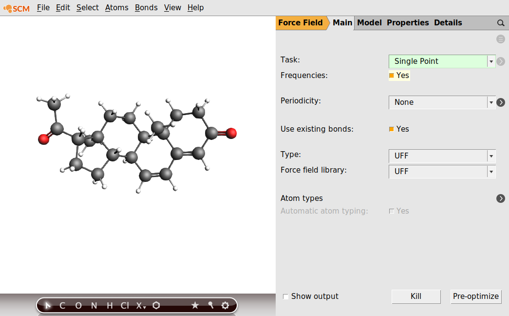
1. Return to the AMSinput window that has the optimized geometry of dydrogesterone.

2. Select the ForceField panel: →

3. Select Task → Single Point and make sure that Frequencies is still enabled on the Properties → Frequencies, … panel.

Note

We have to switch the Task to a Single Point calculation here. For Mode Refinement the calculation of the approximate normal modes should always be done at the equilibrium geometry of the target level of theory, in our case DFTB.

Your AMSinput window should now look like this:

1. Click on File → Save As… and give it the name “UFF_FREQ”.

2. Click on File → Run . This will bring the AMSjobs window to the front.

3. Wait for the calculation to finish. It should be almost instantaneous.

4. Click on SCM → Spectra.

AMSspectra will give a warning that the spectrum is a flat line. This can be explained because by default UFF does not use charges, and hence the dipole is always exactly zero, and consequently also the intensities. For that reason AMSspectra shows the normal mode count. Make the width a bit broader, say 20.

We should now have our approximate modes from UFF in AMSspectra.

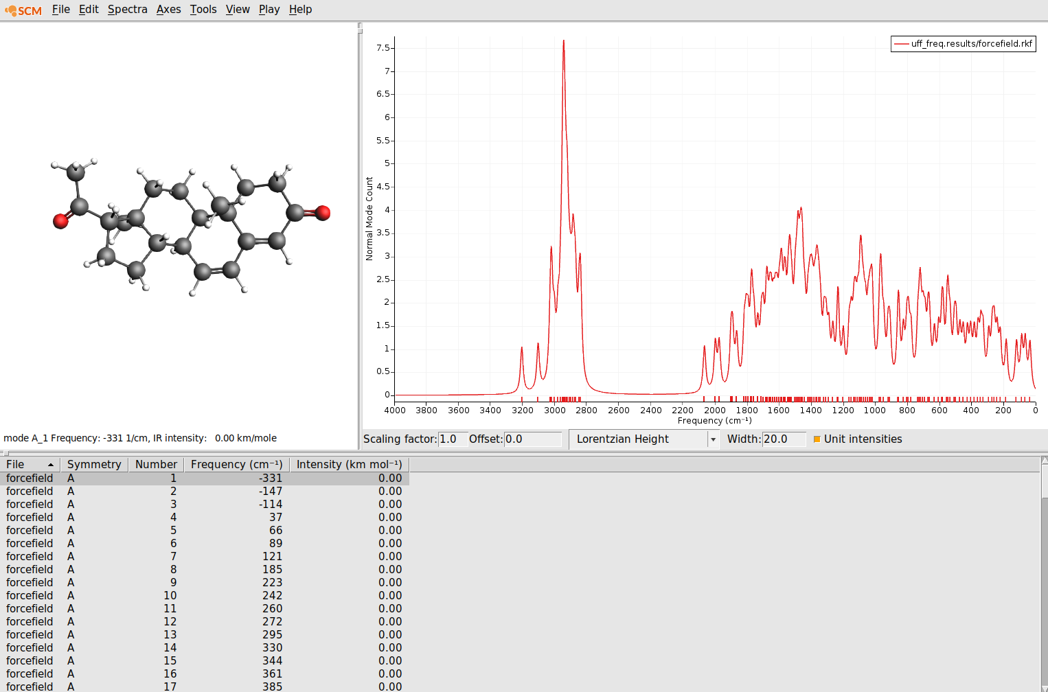
While the C-H stretch band is also separately visible in the UFF spectrum, we can not really see the C=C/C=O stretches and the collective bending modes as distinct bands, as we could in the DFTB spectrum. Note that UFF does not give us IR intensities, and we just have the number of normal modes on the y-axis here.

We will now use Mode Refinement with DFTB on the approximate UFF modes to obtain only the high energy end of the DFTB spectrum.

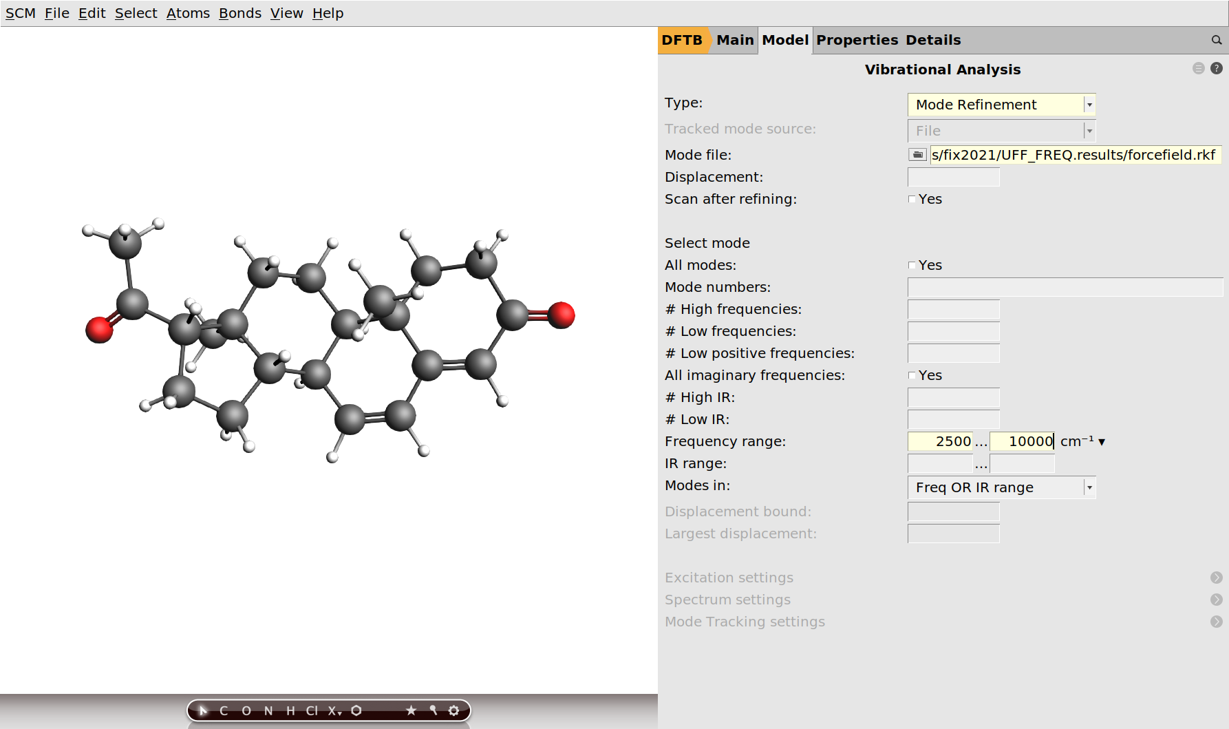
1. Return to the AMSinput window that has the optimized geometry of dydrogesterone.

2. Switch back to the DFTB panel: →

3. Select Task → Vibrational Analysis and disable the Frequencies checkbox.

4. Go to the panel Model → Vibrational Analysis.

5. Select Type → Mode Refinement.

6. Select the approximate UFF modes by selecting the UFF_FREQ.results/forcefield.rkf file in the Mode file field.

Let us as a first step just target the C-H stretch region, and see if we can reproduce the DFTB spectrum in this region. For this we select all modes with frequencies >2500cm^-1 from the UFF spectrum. This covers the entire C-H stretch region in the UFF spectrum, and we should therefore have a good basis of normal modes in which to express the DFTB normal modes we are looking for.

1. Select Frequency range → 2500 … 10000 cm^-1.

We are now ready to run the Mode Refinement job and inspect the results.

1. Click on File → Save As… and give it the name “MR2500+”.

2. Click on File → Run . This will bring the AMSjobs window to the front.

3. Wait for the calculation to finish. It should be almost instantaneous.

4. Click on SCM → Spectra.

5. Click on File → Add… and select DFTB_GOFREQ.results/dftb.rkf.

We now have the reference DFTB spectrum (in blue) as well as the result of the Mode Refinement (red) in the same plot. Zooming into the C-H band, we can compare the results.

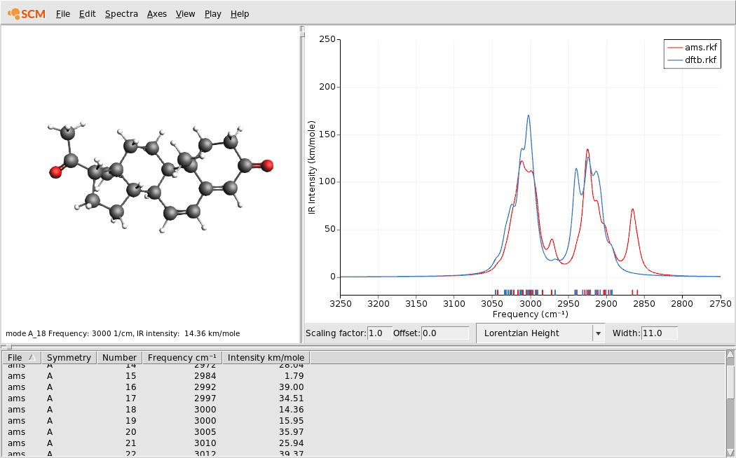
The overall shape, position and intensity of the band is well reproduced by the Mode Refinement, though there is a small extra peak around 2860cm^-1, which does not match the full DFTB spectrum.

Let us increase the size of the basis for the Mode Refinement in order to also get the C=C/C=O stretch band seen in the full DFTB spectrum. In the UFF spectrum we calculated earlier, it is not clear where the C=C/C=O modes are. As such we don’t know precisely what modes from the UFF spectrum to include in our basis. Nevertheless, we can just select a large enough part of the spectrum and hope that the resulting basis is suitable to express the C=C/C=O stretch modes we are looking for. For this tutorial we will use all UFF modes with frequencies >1200cm^-1 as our basis, but we encourage users to play with this value and observe the effect on the resulting spectra.

1. In the AMSinput window of the Mode Refinement job, change the Frequency range to 1200 … 10000 cm^-1.

2. Click on File → Save As… and give it the name “MR1200+”.

3. Click on File → Run . This will bring the AMSjobs window to the front.

4. Wait for the calculation to finish.

5. Click on SCM → Spectra.

6. Click on File → Add… and select DFTB_GOFREQ.results/dftb.rkf.

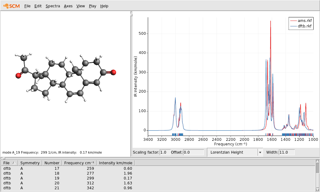
The C-H stretch band is now basically perfect, indicating that UFF modes from <2500cm^-1 region still have some contribution to the C-H stretch band at the DFTB level. The four peaks of the separate C=C/C=O stretch band are also reproduced, though there still some small deviations in peak position. The beginning of the band of collective bending modes is also reproduced very accurately.

It should be noted that this tutorial actually shows a rather difficult case for the Mode Refinement: The UFF modes are quite different from the DFTB mode we wanted to calculate. Therefore a relative large part of the UFF basis is needed to perfectly reproduce the DFTB spectrum. Much better results can be obtained if the approximate and target methods are more closely related (e.g. DFT/DFTB or DFT/DFT with different basis sets). We encourage users to repeat this tutorial using DFT/TZP/BP86 and DFTB3 as target and approximate method. Both methods have a distinct C=C/C=O stretch band in dydrogesterone, which can be picked out in the DFTB spectrum to predict just this band at the DFT level, without calculating the higher energy C-H stretch band. This calculation is demonstrated in this example from the AMS manual, and was also performed in the original article on Mode Refinement.

This concludes the tutorial on Mode Refinement in AMS.