Automated reaction pathway discovery for hydrohalogenation

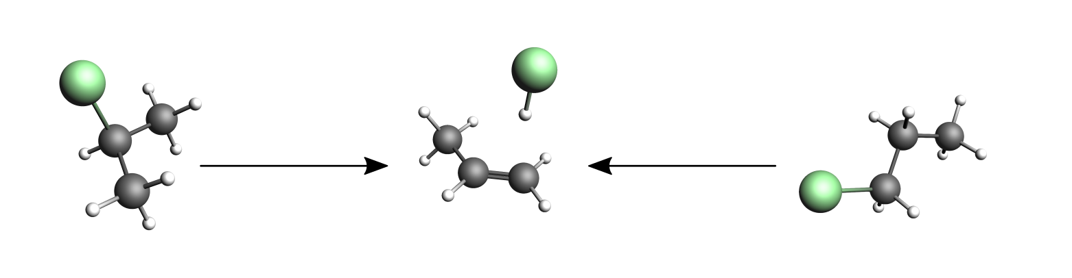
In this tutorial we will use the DFTB engine and the PES exploration task in the AMS driver to study hydrohalogenation. Specifically we will look at the formation of chloropropane from hydrogen chloride and propene:

We will computationally confirm Markovnikov’s rule by discovering and comparing the reaction pathways for both the formation of 1-chloropropane and 2-chloropropane. Markovnikov’s rule states that the halogen atom is preferentially attached to the carbon with fewer hydrogen substituents, i.e. the formation of 2-chloropropane would be preferred over the formation of 1-chloropropane.

Setup of the process search job

The PES exploration task in AMS has various subtasks called “jobs”. In this tutorial we will use the process search job. The process search will start in a local minimum on the potential energy surface (PES) and starting from a random displacement will attempt to find a nearby saddle point (transition state). If a saddle point is found it will cross the saddle and perform a geometry optimization on the other side of the saddle to find a new minimum. This process is repeated a number of times, starting from all the local minima discovered so far. Over time this builds a graph of critical points on the PES, containing information on which minima are connected by which transition states.

We can start the PES exploration in any known local minimum. For this tutorial’s application already know two local minima: 1- and 2-chloropropane! We will just start the process search in these two minima. It should then find hydrogen chloride and propene as well as the processes connecting them to 1- and 2-chloropropane by itself.

We can easily obtain a 1-chloropropane molecule from the structure database in AMSinput:

1. Start AMSinput.

2. In AMSinput, select the DFTB panel: → .

3. Click on the magnifying glass .

4. Search for 1-chloropropane and select C3H7Cl: 1-Chloropropane (ADF) from the list.

We can now copy it and build ourselves a 2-chloropropane molecule by moving the chlorine atom to the central carbon.

1. Select all atoms by pressing Ctrl + a and copy them with Ctrl + c.

2. In the menu bar, click Edit → New Molecule.

3. Insert the copied atoms by pressing Ctrl + v.

4. Grab the chlorine atom and drag it (right mouse button) to the central carbon atom.

5. Grab the a hydrogen from the central carbon atom and drag it to where you removed the chlorine atom.

6. Press the Pre-optimize button on the bottom right of the DFTB panel.

The pre-optimization should fix both the bonds as well as result in an optimized 2-chloropropane structure.

Note that a 2-chloropropane molecule could also be found in the structure database in AMSinput. However, we can not use that one. The PES exploration tasks in AMS require that the mapping from atom indices to atomic species is the same for all input systems. Since the chlorine atom is atom 4 in the first structure (you can check by clicking View → Atom Info → Name → Show), we have to make sure that this is also the case for all other structures in the input. By moving atoms we make sure that the atom index to species mapping remains consistent across all input systems. (If you think about the input states’ geometries as simple xyz-files, then you must be able to convert one to the other just by changing the coordinates, not by exchanging whole lines.)

Warning

For PES exploration jobs with multiple input systems the mapping from atom indices to atomic species has to be the same for all input systems. To ensure this, we recommend that further input systems are built from the original system through the movement of atoms.

If this is not possible, you can see the indices of the atoms by clicking in the menu bar on View → Atom Info → Name → Show. It is possible to change the order of the atoms in the Coordinates panel (in the panel bar: Model → Coordinates) using the Move atom(s) option.

Now that we have both our input structures, we can set up the PES exploration job:

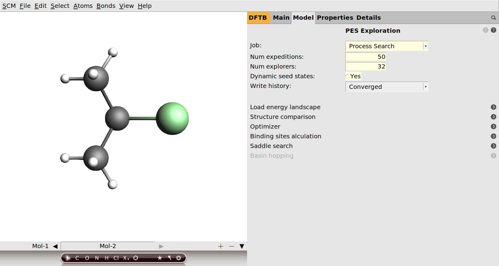
1. Select Task → PES Exploration.

2. Click the button next to the selected task.

3. On the PES Exploration page, select Job → Process Search.

4. Set Num expeditions to 50.

5. Set Num explorers to 32.

As you can see from the right panel in AMSinput, the PES exploration task has a fair amount of options that can be tweaked. Details on the different settings can be found in the PES exploration page in the AMS driver manual. For the purpose of this tutorial we will leave everything at the default values, except the number of expeditions and the number of explorers per expedition.

These two parameters control how thoroughly the PES will be explored. They will determine the run-time of the job, but also affect the number of minima and transition states you will find. Every expedition starts in a specific local minimum and consists of a number of explorers that will independently try to escape from it. A good illustration of the concept of expeditions and explorers can be found in the overview page on PES exploration in the AMS driver manual.

Since all the explorers within one expedition are independent, we can parallelize the calculation by running multiple explorers at the same time. It is therefore recommended to choose the number of explorers equal or larger to the number of available CPU cores. The more expeditions you perform, the larger is your probability of discovering specific processes. As later expeditions may start from minima discovered in earlier expeditions, performing more expeditions will also give you a chance to discover states that are “further away” (by number of intermediate transition states and minima) from the starting point. Unfortunately, it is difficult to predict how many expeditions will be needed to ensure a sufficiently thorough exploration of the PES. Luckily you can view the results of an exploration already while the job is still running, and can interactively stop the exploration when you are satisfied with the states it has found. It is therefore recommended to choose the number of expeditions conservatively large. For this tutorial 50 expeditions of 32 explorers each should be enough to discover the processes we are looking for.

This concludes the setup of the job. We can now run it!

Click File → Run. When asked, give the job the name process_search.

AMSjobs will come to the front and show your running job and the last two lines from its logfile.

There is not much you can tell from seeing just the last two lines, but you can click on them to open the logfile in AMStail, where you can watch the progress of your job.

You will first see the initial optimizations of the input systems 1- and 2-chloropropane, which will be the first states inserted into the database. Afterwards you will see the expeditions and individual explorers. You will probably not see all 32 explorers in each expedition in the logfile. This is a technical consequence of the parallelization over explorers and no cause for concern. (You only see the explorers executed by the first group of cores.) Details on the parallelization over explorers are printed once during the first expedition.

After an expedition is finished you will see the number of minima and transitions states discovered by that expedition. Do not worry if expeditions finish without new states: it depends on the number of explorers per expedition, but with the 32 explorers used in this tutorial, you will probably only find new states every couple of expeditions.

Visualization of the results in AMSmovie

We can look at the states found so far by opening AMSmovie.

Click SCM → Movie to open the AMSmovie module.

You should a graphical representation of the states you have discovered so far in the right panel. Minima are shown with a black level, while transition states are shown using a red level. If you have not found any new processes yet, your energy landscape will probably only consist of the input systems 1- and 2-chloropropane. Let the job run for a while and wait for some processes to be found. The graph on the right will automatically update as your running job finds more states in the background.

When many states are discovered the graph on the right can become a bit messy and overwhelming:

You may for example discover processes that you are simply not interested in, and may wish to hide them in order not to clutter the view. Furthermore the automatic layout of the graph is likely not perfect and you may want to move some states. Luckily there are a number of tools that allow you to edit the graph on the right.

1. Increase/decrease the overall horizontal spacing with Ctrl + ] and Ctrl + [.

2. Select a state by clicking on its energy level. It will be highlighted in blue.

3. Move the state left and right by pressing Ctrl + ← and Ctrl + →.

4. Hide the state by pressing Ctrl + Delete.

5. Restore the hidden states by clicking Energy Profile → Restore Levels.

You can find all these options in the Energy Profile menu at the top, but the hotkeys are worth learning if you frequently work with these graphs. Once you have found a layout that you like, you can also save it.

1. Click Energy Profile → Save Layout.

2. Just for testing make some more changes to your layout.

3. Click Energy Profile → Load Layout to restore the layout you saved earlier.

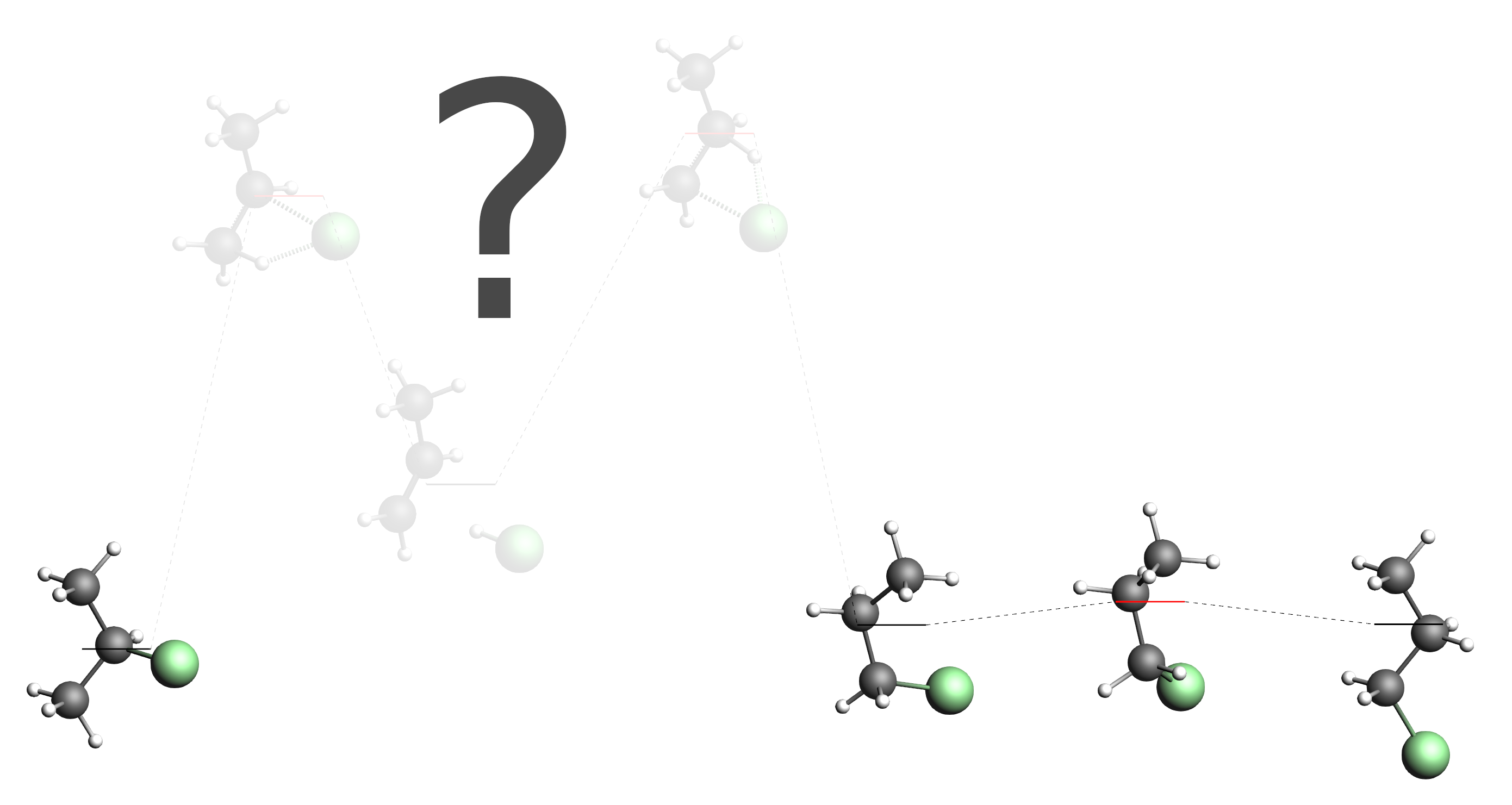
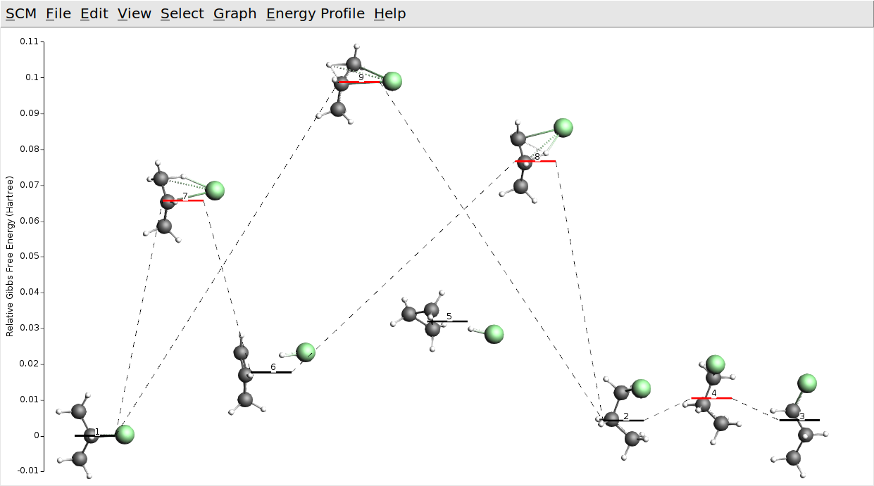
Keep your job running. With a bit of luck you will find all of the following processes after a while:

Note that our input systems on the very left (2-chloropropane) and the very right (1-chloropropane) of the picture above. We have also found another conformer of 1-chloropropane (third from the right). This more “compact” conformer of 1-chloropropane has a slightly lower energy than the “straight” conformer we had in the input. Of course the two conformers are only separated by a very low barrier corresponding to the rotation around the central single bond. As the third from the left we can see the minimum that is separate hydrogen chloride and propene. Note that 2-chloropropane has a slightly lower free energy than the “compact” conformer of 1-chloropropane. Also the barrier from hydrogen chloride to 2-chloropropane is lower than the barrier to 1-chloropropane. This confirms Markovnikov’s rule, stating that the production of 2-chloropropane is preferred.

You may also find a transition state connecting 1- and 2-chloropropane directly, but the barrier for this is higher than for the two step process with hydrogen chloride in the middle.

Note that normal modes have been calculated for all states in the energy landscape. As usual the normal modes can be visualized in AMSspecta.

1. Right click on a line representing an energy level.

2. From the context menu, select Open in module → Spectra.

If you have found the direct conversion between 1- and 2-chloropropane, open the connecting transition state in AMSspectra. The DFTB calculated bonds in the picture above suggest it already: you will find that the direct conversion happens via a transfer of the hydrogen opposite of the chlorine atom.

You can download the movie here if it does not play in your browser.

The PES exploration is a stochastic in nature and you may not discover all the processes shown above. Our testing of this tutorial showed that the probability of finding all of the above processes is about 50%. It is very likely you will discover some of the processes shown above though. Do not worry if you are missing something. The PES exploration can be restarted and you can give it some hints on where to look for new processes. We will learn how to do that in the next section.

While you may not find all the processes shown above, you may find many others! There are for example many processes that decompose the system and split off H₂ or CH₄.

The barriers for these processes are higher though, so we suggest just hiding them all in AMSmovie.

If your process search job is still running in the background and you are satisfied with the states it has found, you can stop it from AMSjobs:

1. Switch to the AMSjobs window.

2. Select the still running process search job.

3. In the menu bar click Job → Request Early Stop.

Note that requesting a job to stop early is different from just killing it. Killing is immediate and forces the stopping at the level of the operating system, while the request to stop early is handled inside the AMS driver and may do different things depending on the task running. Details can be found in the AMS driver manual in the section on the interactive input file. For PES exploration the early stopping will allow all explorers that have already been dispatched to finish and will still incorporate their found states into the energy landscape (and sort all states by energy). This “soft stopping” ensures that the energy landscape is correct and consistent, while just killing the job might leave it in an inconsistent state that you might not be able to restart from.

Restarting a PES exploration

The energy landscape that is visualized in AMSmovie is the primary result of any PES exploration job. However, the the energy landscape is not only the output of a job: it can also be used as input for other PES exploration jobs. This can be used to effectively restart a PES exploration from states discovered in a previous exploration. Let us demonstrate this on the hydrohalogenation example.

Depending on how lucky you were in the first step of this tutorial, you may not have found all of the main processes discussed earlier. Let us pretend that all you found is the conversion between the two conformers of 1-chloropropane, the “straight” conformer we had as input and the “compact” conformer. (If that is not the case for you, you can adjust the following instructions to suit your situation. If you did discover all the main processes but still want to follow this tutorial, you can just hide some of them in AMSmovie and pretend you did not discover them.) Together with the 2-chloropropane molecule that you already provided as input, you would have the following energy landscape:

As you can see, our energy landscape is not connected yet, as we did not yet discover any processes that would connect 2-chloropropane with the 1-chloropropane conformers. In AMSmovie this situation may look like this (hide/delete all unrelated states if necessary):

Note the state numbers on the levels. (You can click the picture above if they are too small to see.) From left to right they are: 1, 2, 4 and 3. We will now set up a second process search, that loads this energy landscape and explores the region around state 1 (2-chloropropane) and state 2 (“compact” conformer of 1-chloropropane).

1. Open the process search job we set up earlier in AMSinput.

2. Immediately save it under a new name by clicking File → Save As…. Call it process_search_restart. (It needs to be a new job so we do not overwrite the results we want to restart from.)

3. Go to the panel: Details → PES Exploration Load Energy Landscape

4. Click the folder button next to Load Energy Landscape From and select the process_search.results folder produced by the previous job.

5. Tick state 1 and 2 as seed states.

6. Optional: Select a subset of states to load, e.g. states 1 to 4.

While loading an energy landscape you can also choose to load only selected states into the new landscape. For this tutorial the step is optional, but you could use it to get rid of states and processes you do not care about.

In the PES exploration the seed states are those minima that may be used as the starting point of an expedition. We selected states 1 and 2 here, since we would like the PES to be explored around these minima. After all, we expect that there should be processes connecting the two states via another minimum (hydrogen chloride and propene) still to be discovered. Normally during a process search the set of possible seed states is expanded as new minima are found. This is the reason why the process search can find minima that are not directly connected (via just one transition state) to the structures provided in the input. Sometimes this is not the desired behavior. For this restart it may make sense to only start expeditions from state 1 and 2 and not add new minima as seed states during the exploration. In this way the exploration stays focused on the region we are interested in and can not wander off exploring unrelated processes. The option to disable the dynamic adding of seed states can be found on the main PES exploration panel.

1. Go to the panel: Model → PES Exploration

2. Untick the Dynamic seed states checkbox.

You can now save the job and run it. If you open it in AMSmovie, you will see that the energy landscape is already populated with the states you loaded from the previous job. Not that you will only discover processes (new minima connected via a transition state) involving the seed states we have chosen. If you keep it running for a while, it is very likely you will “bridge the gap” in your graph through the discovery of hydrogen chloride and propene!

Obtaining the reaction path with the IRC (intrinsic reaction coordinate) method

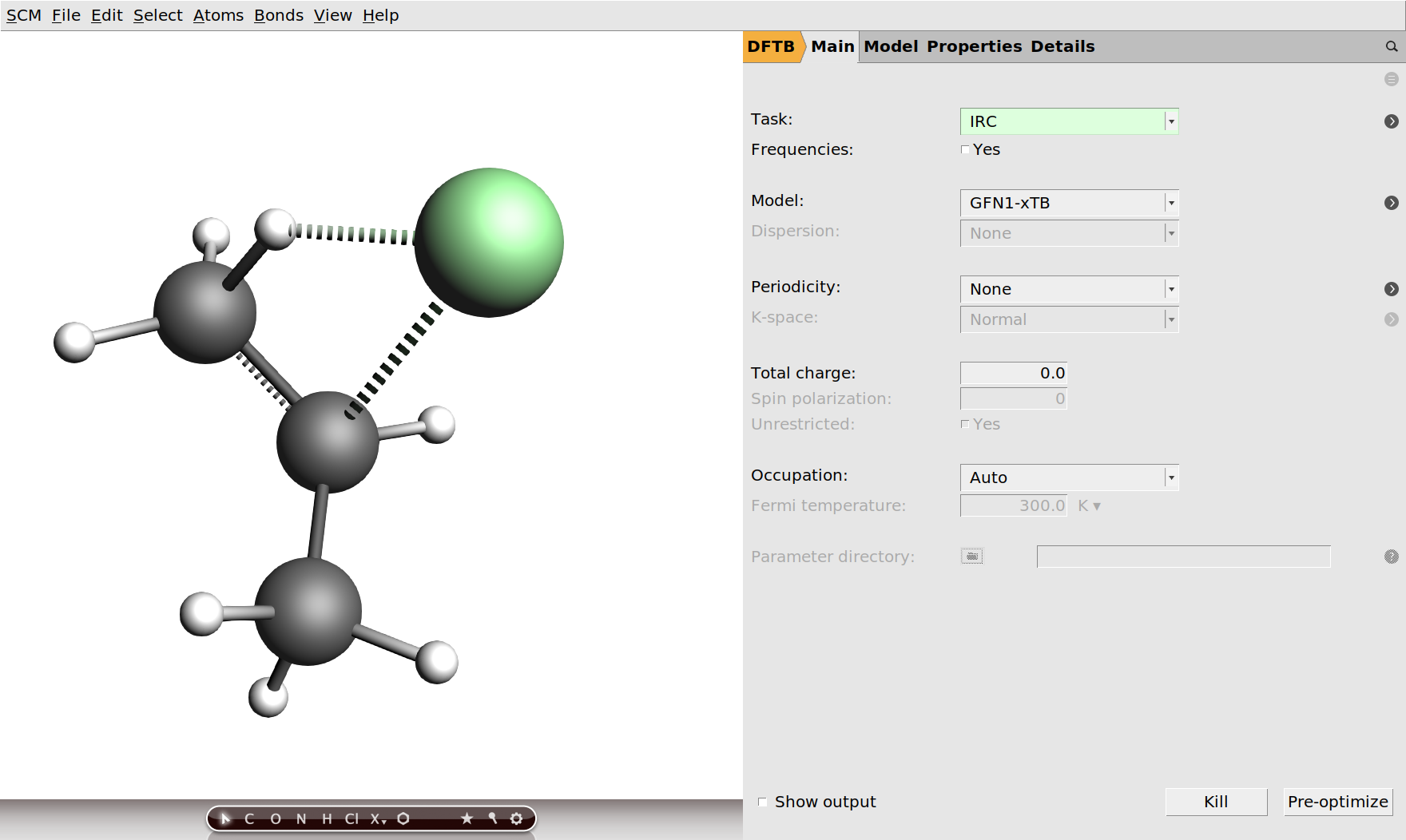
Given the reactants, products and the transition state, you can already get an idea of the reaction process. Nevertheless, it is very nice to be able to visualize the reaction as a movie and to be able to see an energy profile along the reaction path. Since we already have the transition state, this can very easily be done with the intrinsic reaction coordinate (IRC) method in the AMS driver. Let us do this now for the reaction from hydrogen chloride and propene to 2-chloropropane.

1. In AMSmovie, right click the transition state and select Copy Geometry from the context menu.

2. Open a new AMSinput window by clicking SCM → New Input in the menu bar.

3. Paste the geometry of the transition state into AMSinput by pressing Ctrl + v.

4. Switch to the DFTB panel: → .

5. Select Task → IRC.

6. Save and run the job.

Running the job should only take a few second. When it is finished, open the results in AMSmovie.

You can jump around on the reaction path by clicking into the graph, using the slider below the molecule viewport, or via the controls next to it. Your movie should look like this:

You can download the movie here if it does not play in your browser.

Refining an energy landscape at a higher level of theory

The automated PES exploration in AMS can be computationally quite demanding. It is often not feasible to perform it directly with higher level methods like DFT. However, the results of a PES exploration at a lower level of theory can be used to give you an idea of the processes that may exist, which you could then study “manually” at a higher level of theory. You may for example take two minima and the connecting transitions state from a lower level of theory and use them as input for a NEB calculation with DFT. This may already be quite expensive.

A cheaper and still useful alternative would be to just reoptimize all the states found at the lower level of theory with a higher level method. For local minima this would mean a simple geometry optimization, while all the transition states would serve as input for a transition state search. This workflow is implemented as one of the subtasks of the PES exploration in the AMS driver, where it is called energy landscape refinement. Let us use it now to bring the DFTB results we obtained earlier to the DFT level!

We assume that by now you have found some interesting processes, e.g. the formation of chloropropane from hydrogen chloride and propene, the two 1-chloropropane conformers, and the direct conversion between 1- and 2-chloropropane. In AMSmovie you may see something like this:

Your process searches may also have found cyclopropane and hydrogen chloride, which we have kept in the picture above (state 5). Note that with GFN1-xTB it is actually lower in (free) energy than propene and hydrogen chloride (state 6). This seems to be wrong. Let us check if that is still true at the DFT level.

1. Open AMSinput by clicking: SCM → New Input

2. On the main ADF panel, set the XC function to GGA-D → PBE-D3(BJ).

3. Set the Basis set to TZP.

4. Select Task → PES Exploration.

5. Click the button next to the selected task.

6. On the PES Exploration page, select Job → Landscape Refinement.

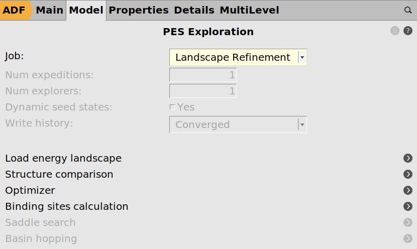
7. Cick the next to Load Energy Landscape.

8. Click the folder button next to Load Energy Landscape From and select the results folder with the energy landscape you want to refine.

9. Optional: Select individual states from the energy landscape to load. We suggest you refine at least the states involved in the main processes as well as the cyclopropane state.

10. Save and run the job.

You can watch the process of the optimizations and transition state searches in AMSmovie while the job is running. As soon as the first state has been refined, you can also watch your energy landscape graph “grow” in AMSmovie. (You can switch back and forth between the two views with View → Energy Landscape States in the menu bar of AMSmovie.)

Once your job has finished, your DFT refined energy landscape may look like this:

Except for the relative ordering of cyclopropane and propene the DFT energy landscape is not qualitatively different. All barriers seem to be a bit lower with DFT though. Note that the semi-empirical GFN1-xTB model we used is optimized for structural properties (Geometries, Frequencies, and Non-covalent interactions). In view of this, we may forgive these inaccuracies for total and reaction energies.