Transition state search and characterization of a Ziegler Natta Catalyst

Introduction

Ziegler-Natta catalyzed polymerization

In this tutorial, you will learn how to locate the transition state (TS) for the insertion step of ethylene polymerization catalyzed by a homogeneous Ziegler-Natta catalyst.

Discovered by Karl Ziegler and first applied to polymerization by Giulio Natta, this class of catalysts soon became an industry standard for the production of various polyolefins. Consequently, Ziegler’s and Natta’s work was awarded a Nobel Prize in 1963. Nowadays, the industrial Ziegler-Natta polymerization of polyolefins is among the most important industrial processes.

In the following tutorial, we use the AMS driver and DFTB to locate and characterize the transition state of a Ziegler-Natta reaction and use these results to calculate an approximate rate constant. You are also encouraged to learn how to reuse these results to expedite follow-up ADF calculations for more accurate results.

Strategy

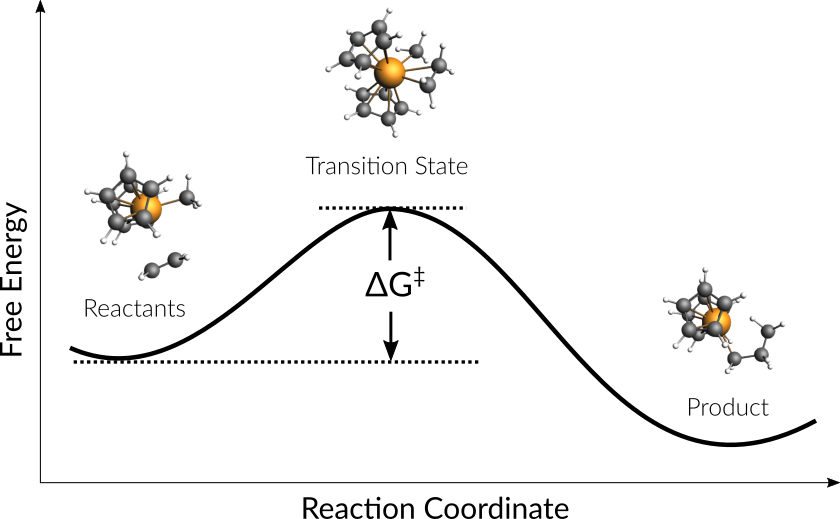
Consider the following Ziegler-Natta reaction:

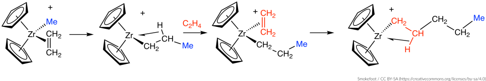
We will use a two-stage approach to locate the transition state of this reaction:

• Find an initial guess of the TS by scanning the potential energy surface (PES scan) along the bonds newly formed during the reaction (we will use a composite coordinate scan).
• Optimize and characterize the initial TS guess (transition state search).

Geometry Setup with AMSinput

This section shows how to construct the geometry of the ethene-metallocenium (Cp₂Zr⁺CH₃- C₂H₄) complex in AMSinput.

Import geometry from xyz file

Build the structure yourself

1. Download the xyz file of the ethene-metallocenium complex

2. In AMSinput select File → Import coordinates and select the file you just downloaded

3. Proceed with the Settings for the Engine section

See also

If you are not yet familiar with the editing tools in AMSinput, take a look at our Introduction to Building structures.

In AMSinput

1. Select the ferrocene structure in the structure tool: → Metal complexes → Sandwiches → Ferrocene Sandwich

2. Replace Fe with a Zr: Right-click on the Fe atom → Change atom type → Zr

3. Click on the Zr atom, select the Carbon tool () and add a carbon atom

4. Click on Atoms → Add hydrogens

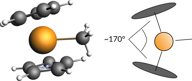
Change the angle between the two benzene rings:

1. Select one of the dummy atoms in the ring center

2. Holding down shift click on the Zr atom and then on the other dummy atoms in the ring center

3. Change the Xx-Zr-Xx angle to 170 (or use the slider)

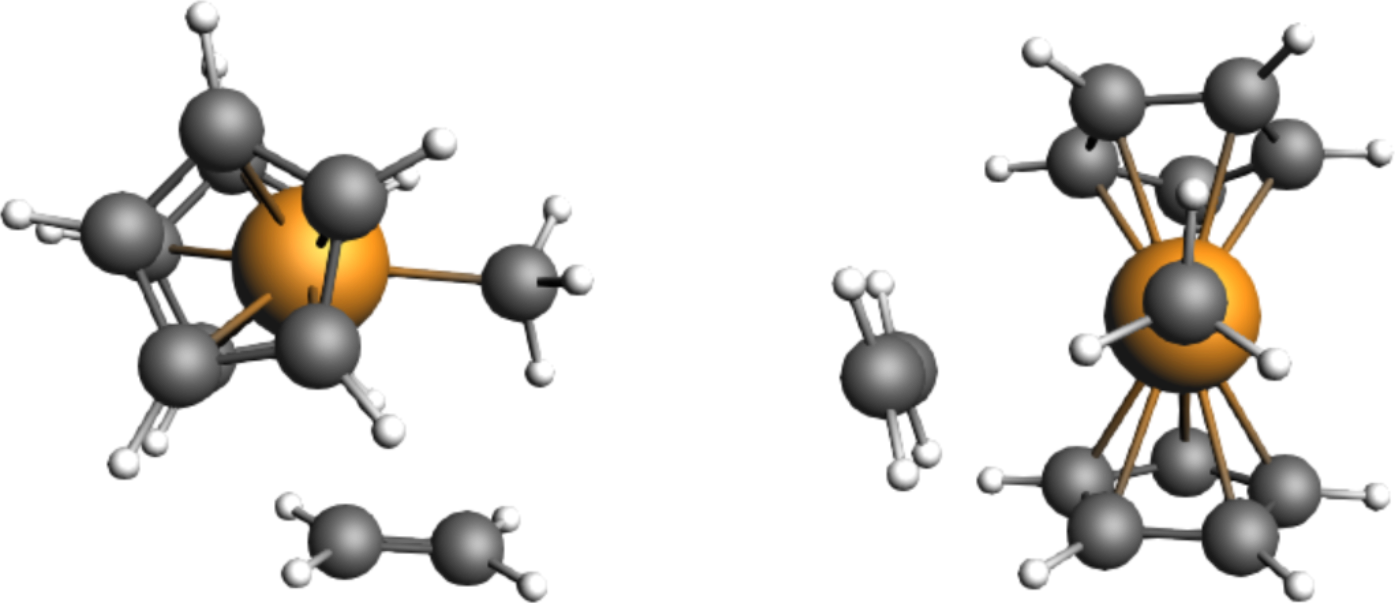
Finally we can add a ethene molecule:

1. In the search box type ethene

2. Select Molecules → C2H4: Ethene (ADF)

3. Position the ethane molecule roughly as shown in the picture below

We now want to pre-optimize the structure we just built:

1. Switch to the DFTB panel: →

2. Set the Total charge to 1

3. Go to the tab Model → Solvation and select Solvent → Toluene

4. Go to the Main panel and click on Pre-Optimize

Settings for the Engine

In the course of this tutorial, the DFTB engine with the GFN-1xTB model and implicit Toluene solvation is used. This particular setup provides a good compromise between computational speed and accuracy well suited for this tutorial. Other engines, such as our DFT code ADF, will yield more accurate results but will require longer computation time.

Here are possible engine settings for this tutorial

DFTB

ADF

MOPAC

For a GFN1-xTB DFTB calculation with implicit Toluene solvation use the following settings:

1. Select the DFTB panel:

2. Set the Total charge to 1

3. Go to the tab Model → Solvation and select Solvent → Toluene

For a DFT calculation with ADF, try the following settings.

1. Select the ADF panel:

2. Set the Total charge to 1

3. XC functional → GGA-D → PBE-D4(EEQ)

4. Basis set → DZP

5. Go to panel Model → Solvation

6. Select Solvation method → COSMO

7. Select COSMO Solvent → Toluene

The pre-optimized geometries provided throughout this tutorial are optimized with DFTB. Make sure to re-optimize them when you switch to ADF.

Tip

To just confirm a TS with ADF, do not run a full frequency calculation! Instead use the much faster PES point characterization available under Properties -> IR (Frequencies) -> Characterize PES point.

For a semiempirical calculation with MOPAC, we suggest starting with following settings

1. Total charge select 1

2. Method → PM7

3. Go to panel Model → Solvation

4. Check the box Use COSMO

5. Solvent → Toluene

Settings for the AMS Driver

First, take a look at the reactants and the product in the following figure to identify the two required scan coordinates:

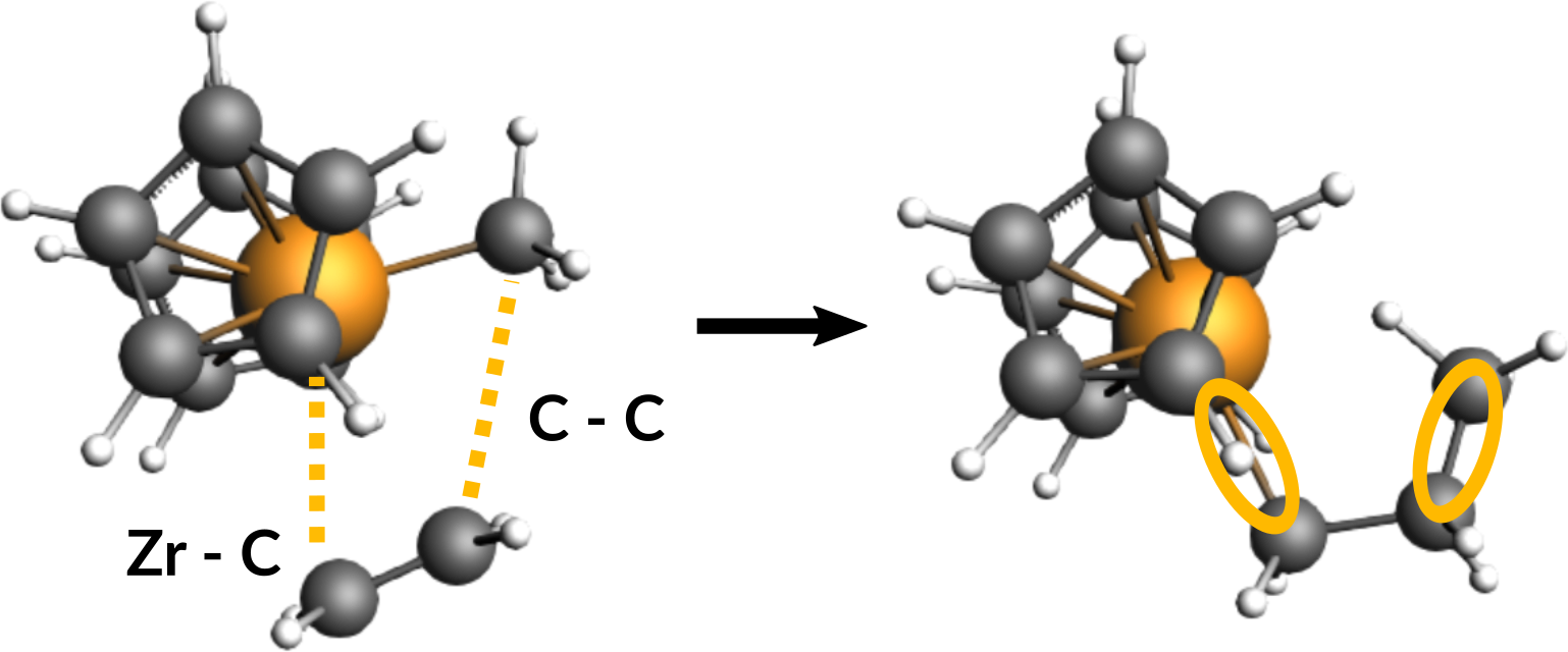
During the reaction, two bonds will be newly formed:

• Zirconium-Carbon (between Zr-Ion and the ethene molecule)
• Carbon-Carbon (between ethene molecule and methyl group)

These two distances will serve as scan coordinates and these will be scanned starting from their present values down to the distance of a typical Zr-C (measured from Zr-Methyl: ~2.3 Å) and Carbon-Carbon single bond (~1.5 Å).

Setup PES scan

To perform a PES scan, change the task in the main panel of the engine:

1. Task → PES Scan

2. Click on next to the Task to specify the scan settings (or Model → Geometry Constraints and PES Scan)

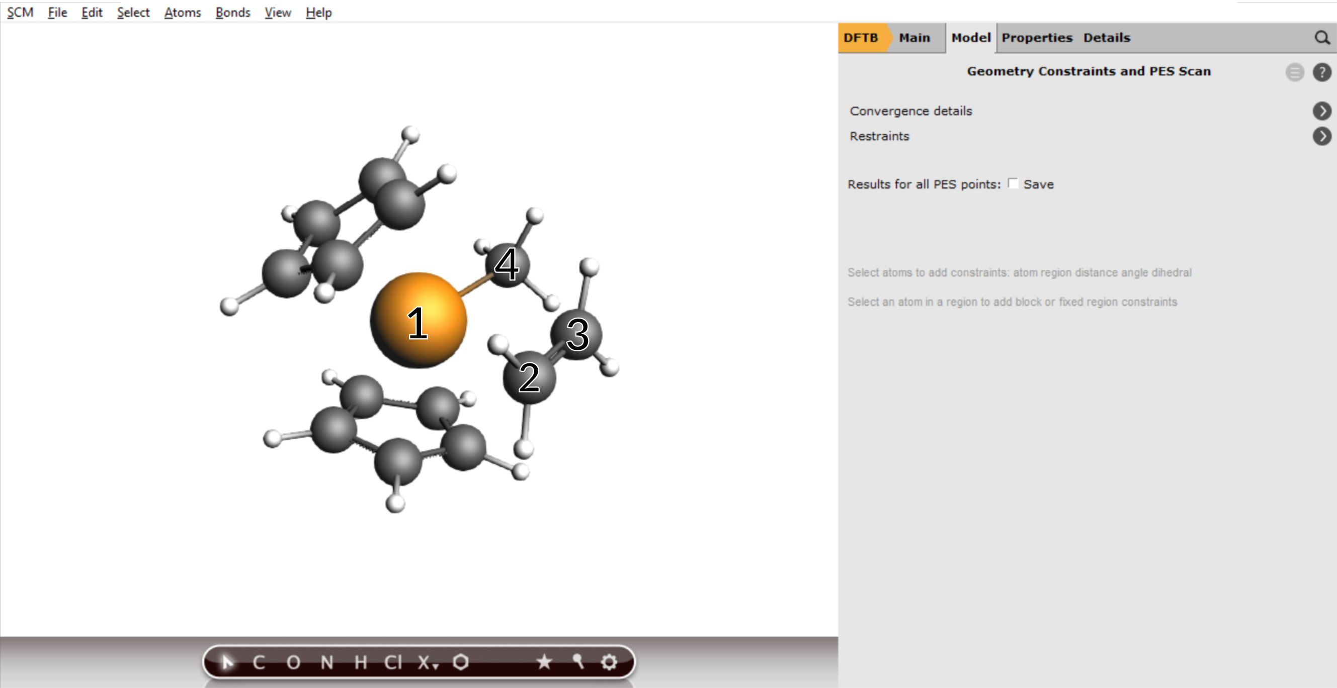
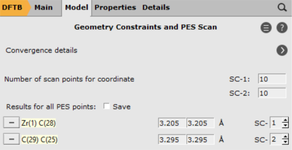
To add a scan coordinate, first select an atom pair

1. Select the Zr (1) and C atom (2). Hold down SHIFT Key for multiple selections.

2. Press the + Button next Zr(..)C(..) distance

3. Enter 2.3 into the second field.

4. Repeat the process for the two Carbon atoms (3) and (4).

5. Enter 1.5 into the second field for the Carbon atoms

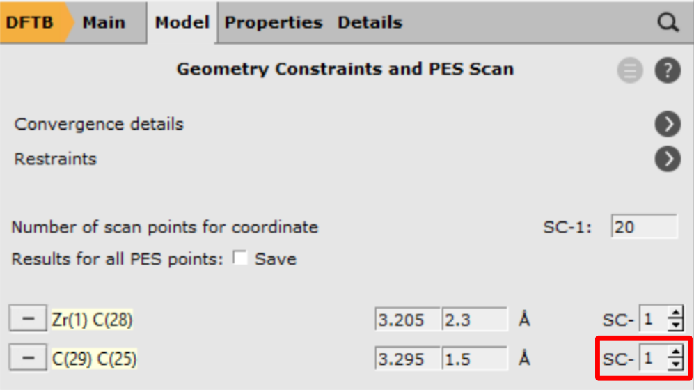
With these settings AMS will scan both coordinates independently, resulting in a 2D projection of the potential energy surface. However, with only one click you can combine the two distances into a single, composite coordinate:

1. Change the SC- index for the C-C distance from 2 to 1

2. Increase the number of scan points to 20

Note

This combination of coordinates implies a concerted formation of bonds. In a situation where this is not known beforehand an independent scan of the two coordinates might yield better results.

In the last step, loosen the convergence criteria of the geometry optimizer, since a fully converged path is not required at this point, but only a guess close to the transition state geometry.

1. Click on next to Convergence Details

2. Soften the convergence criteria by raising the thresholds to:

- Gradient Convergence 0.005

- Energy convergence 5.0e-5

Now you only need to save and run the calculation. The progress can be monitored with AMSmovie.

1. File → Save

2. File → Run

3. SCM → Movie

At runtime, you will see all calculated geometries, including intermediates from the geometry optimizations. Once the PES scan is complete, these intermediates will be hidden. Depending on the AMS version you are using, you might need to close and reopen AMSmovie for this effect to take place. Your plots should roughly look as follows now

Use the scroll bar to navigate to the highest energy structure or click on the highest point in the energy curve. This geometry will serve as the initial guess for the transition state optimization!

From AMSmovie, save the structure with the highest energy

1. File → Save Geometry and give it the name “TS_initial_guess.xyz”

Transition State search

Tip

To ensure an efficient transition state search the starting geometry should be close to the expected TS. It furthermore helps to also have a good guess for the local curvature of the potential energy surface, e.g. from a frequency calculation. The Amsterdam Modeling Suite can provide such initial guesses and offers various methods for locating transition states.

A good overview of further strategies for more specific situations, tips & tricks is given in our slides Hands-On Transition State Search.

See also the AMS manual page on transition state search for more details.

We begin by importing the guess for the transition state saved from the PES scan explained in the previous section into AMSinput.

1. Open a new AMSinput window: SCM → New Input

2. Select the DFTB panel:

3. File → Import Coordinates and select the “TS_initial_guess.xyz” (the file you exported from AMSmovie in the previous section)

4. Change Task to Transition State

5. Check the Frequencies checkbox

Tip

For DFT calculations on large systems, a much faster way of verifying that you found a transition state is the PES point characterization. This can be enabled in AMSinput in Properties → IR (Frequencies) → Characterize PES point.

The settings for the engine are the same as before: GFN-1xTB with a total charge of 1.0 and implicit Toluene solvation:

1. Set the Total charge to 1

2. Go to the tab Model → Solvation and select Solvent → Toluene

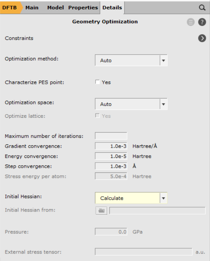
There exist several (approximate) options for the generation of an initial Hessian that is required for the transition state search. In this case, we shall start from the full Hessian evaluated at the initial guess for the transition state structure. This calculation can be requested with the option Calculate in the geometry optimization details panel:

1. Go to Details → Geometry Optimization

2. From the Initial Hessian menu, select Calculate

1. File → Save

2. File → Run

For a well-chosen starting structure, the transition state search should converge to the actual transition state geometry within a few iterations. Once the calculation is finished, open AMSspectra to inspect the calculated frequencies.

1. SCM → Spectra

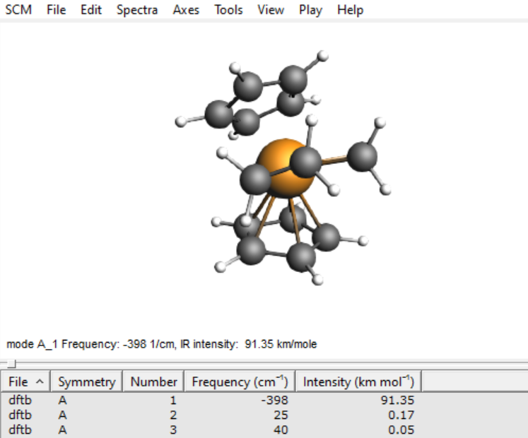
You should see only a single imaginary frequency indicated by a minus sign in the table of frequencies. If you do, then you have successfully optimized the transition state of this Ziegler-Natta reaction.

Tip

One might encounter additional imaginary modes due to either numerical artifacts or very shallow internal modes. In either case, the corresponding frequencies should be small (i.e. around -5 to -25 cm^-1), in which case those modes can be ignored.

Results

Energies and barrier height

Once you have optimized a transition state, you can look at the energies to determine the reaction barrier height. You can find the Energy listed in the output file:

1. SCM → Output

2. Type ‘calculation results’ into the search field at the bottom, next to the magnifying glass and hit ENTER

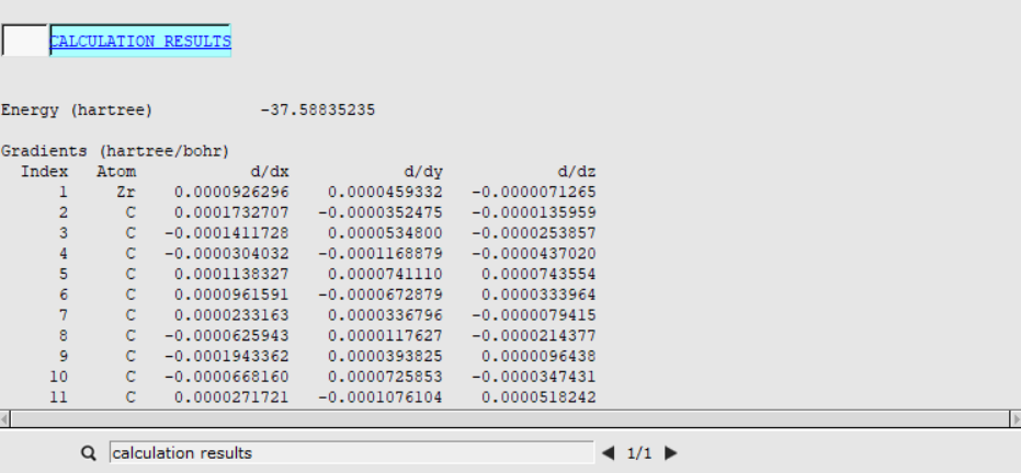
The Energy for the reactants was already calculated when you ran a geometry optimization of the ethene-metallocenium (Cp₂Zr⁺CH₃- C₂H₄) in the AMSinput Geometry Setup. In the corresponding output file it was found to be E_reactants= -37.6079 Hartree.

The barrier height for this reaction can now be calculated as the difference between these two energies \(E_\text{barrier}= E_\text{TS} - E_\text{reactants} = 0.01937 \text{[Hartree]} = 12.26 \text{[kcal/mol]}\)

Kinetics and Statistical Thermal Analysis

When asked to calculate frequencies, AMS will automatically calculate some useful thermodynamic properties such as entropy, internal energy, constant volume heat capacity, enthalpy, and Gibbs free energy from a statistical mechanics partition function. You can find more information on this in the corresponding section of the AMS manual . For now, we shall use these properties to calculate the rate constant.

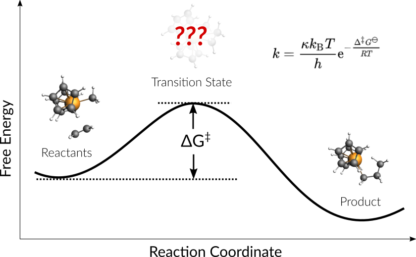
Using Gibbs Free Energy of activation we can estimate the rate constant as described by the Eyring-Polanyi equation:

\[k = \kappa (k_{B}T/h) \cdot \exp \left( \frac{-\Delta G^{‡}}{RT} \right)\]

with the transmission coefficient \(\kappa\) assumed to be 1 (By setting \(\kappa = 1\), the resulting rate formula is commonly known as the Transition State Theory rate. This factor corrects for those reactive trajectories that recross the transition state and return without decomposing. It always reduces the reaction rate, so in general \(\kappa \le 1\)), the rate constant for this single step reaction can be calculated from the Gibbs Free Energy of activation ( \(\Delta G^{‡}\)).

To calculate \(\Delta G^{‡}\) we need to know the Gibbs Free Energy of both the transition state and the reactants.

The Free Energy of the transition state ( \(G_{\text{TS}}\) ) can be found in the thermodynamic properties section of the TS optimization output file:

1. SCM → Output

2. Type Gibbs into the search field at the bottom, next to the magnifying glass and hit ENTER

\[G_{\rm{TS}} = -23460.94 \: \textrm{kcal/mol}\]

For the Gibbs Free Energy of the reactants a frequency calculation has to be carried out. Just download the optimized ethene-metallocenium structure and run a single point calculation to obtain the frequencies

1. Use same engine settings as with previous calculations

2. Task -> Single Point

3. Check the frequencies box under the task menu

4. Once done, search for gibbs in the output file

With a resulting Gibbs Free Energy of

\[G_{\rm{reacs}} = -23475.23 \: \textrm{kcal/mol}\]

the Gibbs Free Energy of activation, \(\Delta G^{‡}\), becomes

\[\Delta G^{‡} = G_{\rm{TS}} - G_{\rm{reacs}} = 14.29 \: \textrm{kcal/mol}\]

and the Eyring-Polanyi rate constant at 295.15 K is calculated as

\[k = 1 \cdot (k_{B}T/h) \cdot \exp \left( \frac{-14.29 \: \textrm{kcal/mol}}{RT} \right) = 214 \, \textrm{s}^{-1}\]

Workflows & Scripting

PLAMS Workflows

Run scripts

This optional section deals with the workflow automation of this tutorial. It assumes basic knowledge about the command line. If you have not used the command line with AMS before, take a look at our information on how to use the command line .

The tutorial splits into two basic steps that can be combined into one but are provided as separate scripts here for the sake of simplicity:

• PES-scan.py runs a PES scan and extracts the highest energy structure as xyz file
• TS-optimize.py uses the structure generated by PES-scan.py as initial guess to optimize and characterize the TS.

To execute the workflow:

1. Download optimized ethene-metallocenium complex and place it into an empty directory.

2. Download PES-scan.py and TS-optimize.py and place into the same directory.

3. Open the command line and type: plams PES-scan.py

4. Once the calculation has finished you can run the second script with plams TS-optimize.py

The scripts are meant to be run after another as the first script generates the input structure for the second script. The results are printed to the command line.

Some results are printed to the command line. All results are found in the binary ams.rkf and dftb.rkf results files.

KF files can be opened and inspected with the GUI program KF Browser. They should only be viewed in Expert Mode:

1. File → Expert Mode

The PLAMS scripts provided above demonstrate how to read results from these files. A short overview of relevant entries is provided in the tables below.

The PES scan calculation results are found in the KF file *.results/ams.rkf

Table 1 Results in the KF file ams.rkf

Section	Variable	Meaning
PESScan	nScanCoord	Number of independently scanned coordinates
PESScan	nPoints(1-nScanCoord)	Number of points scanned for every scan coordinate
PESScan	RangeStart(1 until nScanCoord)	Starting values for scan coordinate 1 (in Bohr)
PESScan	RangeEnd(1 until nScanCoord)	End values for scan coordinate 1 (in Bohr)
PESScan	PESCoords	Coordinates of the PES (in Bohr)
PESScan	PES	Energies of the PES scan (in Hartree)
PESScan	History Indices	Index of PES point geometries in section History

The frequencies calculated after the transition state optimization are found in the engine specific results file. For DFTB this file is called *.results/dftb.rkf:

Table 2 Results in the KF file dftb.rkf

Section	Variable	Meaning
AMS results	Energy	Final energy of the TS (in Hartree)
Vibrations	Frequencies	Sorted list of final frequencies (in cm-1)

The calculations can be run directly from a console input by executing the following run scripts:

• ZN-PES-Scan.run for the PES scan
• ZN-TS-Opt.run for the Transition State optimization

To run the scripts from the command line use the following commands

1. chmod +x ZN-PES-Scan.run

2. ZN-PES-Scan.run > ZN-PES-Scan.out

3. chmod +x ZN-TS-Opt.run

4. ZN-TS-Opt.run > ZN-TS-Opt.out

The results are then found in the corresponding output files ZN-PES-Scan.out and ZN-PES-TS-Opt.out

Note

If you running the scripts produces an error like /bin/sh^M: bad interpreter: No such file or directory, you need to convert the .run script from Windows to Unix line endings first. You can easily do that with dos2unix ZN-PES-Scan.run.