Using the UNIFAC program

The UNIFAC program is an implementation of the UNIFAC method, a fast and accurate liquid-phase activity coefficient model. One of the main advantages of the UNIFAC method is that it does not require any ADF calculations and can estimate thermodynamic properties based only on SMILES strings representations of every molecule in the system (this can also be done with COSMO-RS using FastSigma) . This means that the UNIFAC method can be applied to liquid systems for which no 3D/surface charge information is known. Additionally, UNIFAC is very efficient, able to generate thermodynamic property estimates in milliseconds. In the following sections, we review basic GUI functionality for the UNIFAC program.

Selecting/inputting compounds

Molecules can be used with the UNIFAC program in two ways:

(1) Simply choosing them from the ADFCRS compound database.

(2) Inputting a SMILES string in Compounds → Add Compound using QSPR (Fast Sigma). → Add. This will generate a .compkf file, which will appear in the compound database and can be used with UNIFAC calculations.

Caution

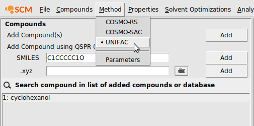
In the current version of the GUI, you can only add a compound by SMILES string if the method COSMO-RS or COSMO-SAC is selected. It will not work if UNIFAC is selected.

To input a molecule as a SMILES string, simply follow the instructions above, typing the SMILES string in the field. As an example, we input cyclohexanol:

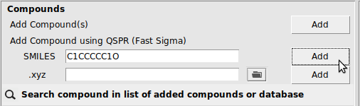
This will prompt you to save your compound as a .compkf file. After saving it, it should appear in the database.

Inputting property values

For some types of UNIFAC calculations, physical property data will be required. For most applications, all of the required physical property data can be input from the compounds menu: Compounds → List of Added Compounds. Property input fields are given in the right panel. As an example, we click estimate to estimate the VPM1 vapor pressure coefficients for cyclohexanol :

Note that other properties (enthalpy of fusion, melting point, etc.) can be input or estimated with a Property Prediction Method.

Calculations with the UNIFAC program

To begin, first navigate to the UNIFAC method:

Start AMScrs (if not already open)

Select Method → UNIFAC

All of the available properties for UNIFAC are listed under Properties →:

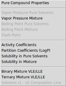
Pure Compound Properties provides estimated physical properties for a compound, but the rest require a UNIFAC calculation. The rest are summarized in the following subsections.

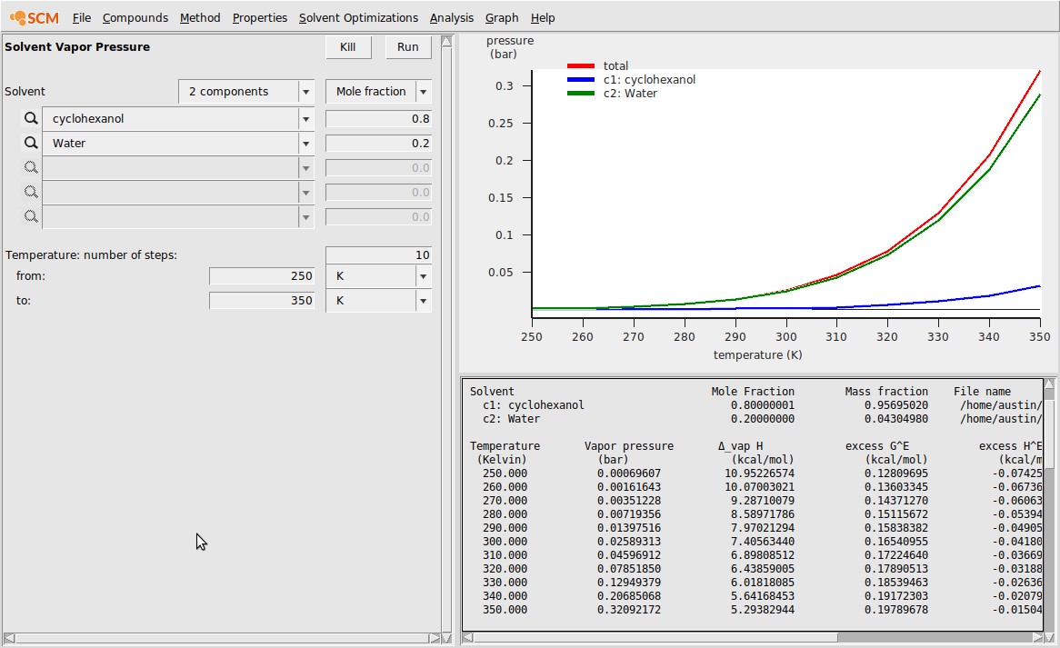
Vapor Pressure Mixture

Properties → Vapor Pressure Mixture

For this calculation, we also select water from the ADFCRS database. We click estimate next to Vapor pressure equation for Water in Compounds → List of Added Compounds. Also, make sure the vapor pressure parameters are already estimated for cyclohexanol (this was done in a previous section). Next, we navigate to the Properties → Vapor Pressure Mixture window. We choose a two component mixture of 0.8:0.2 cyclohexanol:water and change the temperature range to 250-350 K. After hitting Run, we obtain the following:

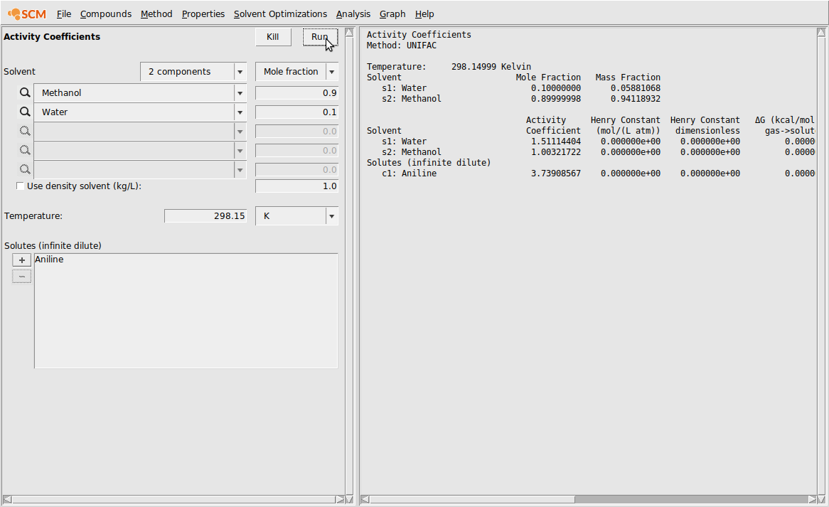
Activity Coefficients

Properties → Activity Coefficients

Next, we demonstrate the activity coefficient calculation module. In this example calculation, we calculate the activities of a 0.9:0.1 Methanol/Water system (both compounds were selected from the ADFCRS database). Additionally, we calculate the activity coefficient of aniline at infinite dilution in this system:

Partition Coefficients (LogP)

Properties → Partition Coefficients (LogP)

In this example, we calculate the logP of Ibuprofen, Thymol, and Xylitol in the standard Octanol/Water system.

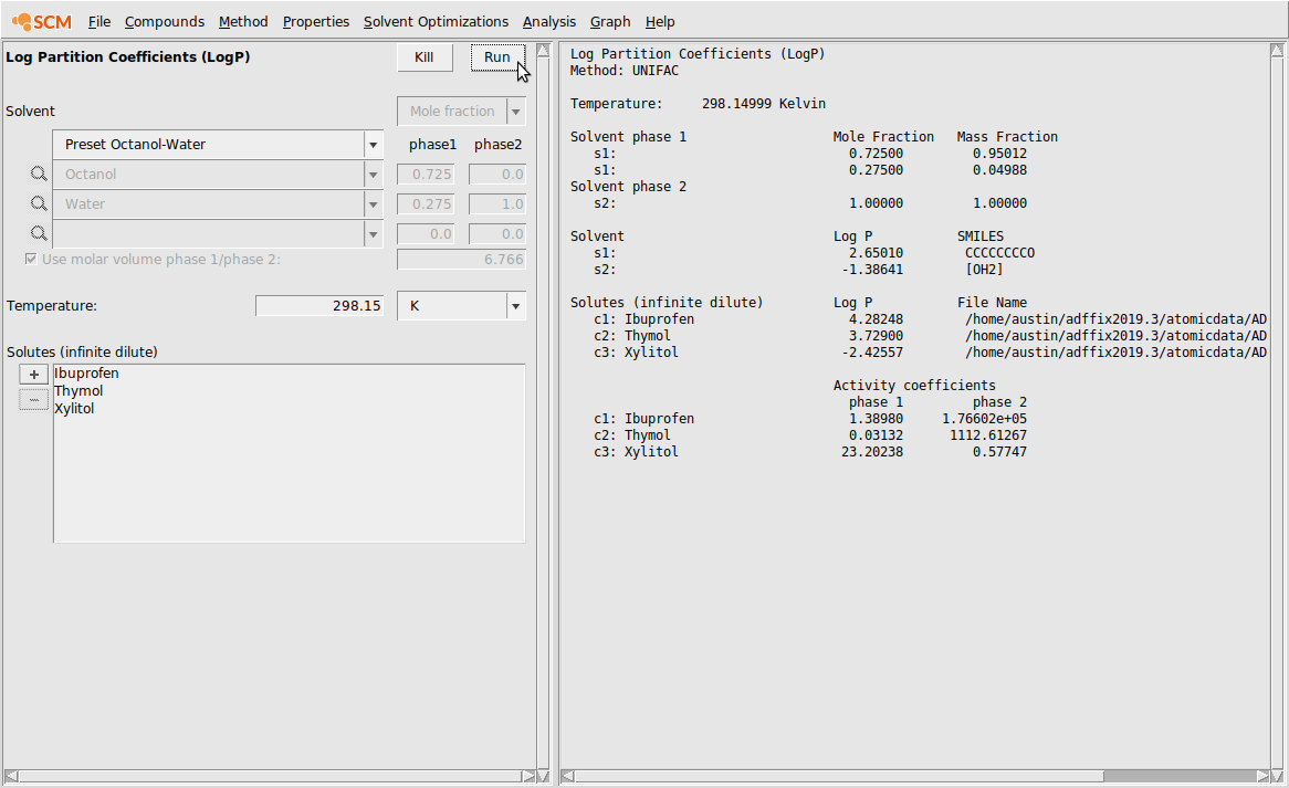
Caution

Only the presets work in the current implementation. User-defined solvent systems will not work.

Solubility in Pure Solvents

Properties → Solubility in Pure Solvents

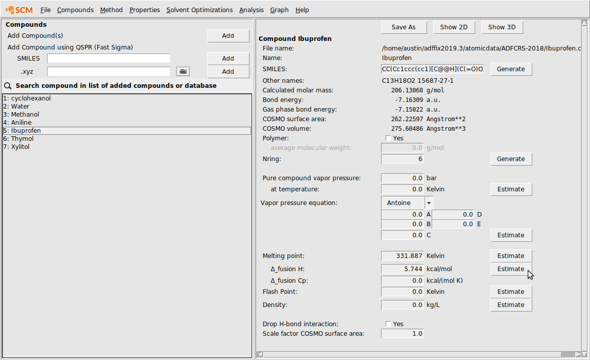
In this example, we calculate the solubility of Ibuprofen in a few different solvents: Methanol, Water, and Cyclohexanol (from our input SMILES string). We also want to consider the solubility over the temperature range 250-298.15 K. Because Ibuprofen is a solid at these temperatures, we require its Enthalpy of Fusion and Melting Point. We can either enter experimental values or estimate the values in the Compounds → List of Added Compounds menu. Even though these properties are known experimentally, we will estimate them as shown below:

Now, we can navigate to Properties → Solubility in Pure Solvents and input the following:

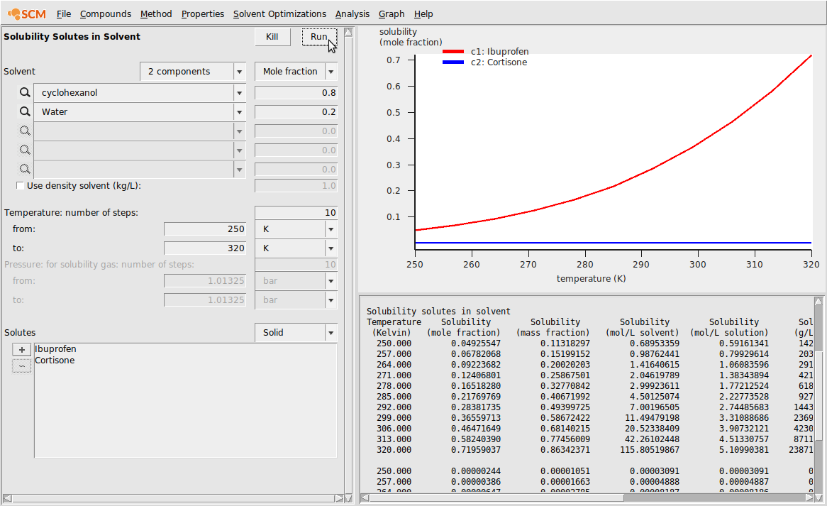
Solubility in Mixture

Properties → Solubility in Mixture

Solubility in Mixture is very similar to Solubility in Pure Solvents. In this case, we specify a mixture of cyclohexanol and water and estimate the solubilities of Ibuprofen and Cortisone in that mixture from 250 K to 320 K. Since Cortisone is also a solid over this temperature range, we first have to estimate its melting temperature and enthalpy of fusion from the Compounds → List of Added Compounds menu. The calculation looks like the following:

Binary Mixture VLE/LLE

Properties → Binary Mixture VLE/LLE

To demonstrate the Binary Mixture module, we again use our cyclohexanol/water system because we’ve already estimated the VPM1 coefficients. If just beginning this tutorial at this step, ensure that both compounds have estimated vapor pressure equations. If vapor pressure information is found, the vapor pressure will be set to 0 and VLE data will not be meaningful. After running the calculation, we adjust the default graph display to view the excess energies. This can be done with Graph → Y Axes → excess energies. The result is the following:

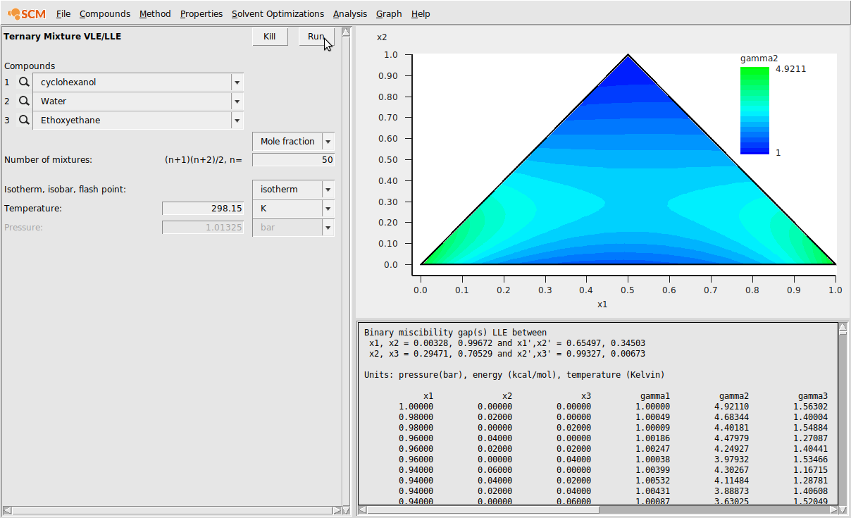
Ternary Mixture VLE/LLE

Properties → Ternary Mixture VLE/LLE

Next, we add a ethoxyethane (diethyl ether) to our cyclohexanol/water system to investigate the behavior of the ternary mixture. Make sure to estimate the VPM1 parameters for ethoxyethane from the Compounds → List of Added Compounds menu. Additionally, we change the number of mixtures to 50.

After running the job, we change the default graph display to a ternary plot with Graph → Triangle \(\boldsymbol \Delta\). Also, the background color has been changed to show the activity coefficient of compound 2 (water) at the different mole fractions. This was done with Graph → Z Colormap → gamma2. This results in the following:

Common issues

The most frequently encountered issue with the UNIFAC program is termination due to lack of binary interaction parameters. Unlike COSMO-RS/-SAC, UNIFAC requires binary interaction parameters for every pair of molecular substructures – called groups – in the mixture. There are many cases where these binary interaction parameters do not exist or are not publicly known. For molecular systems with even one missing interaction parameter, no UNIFAC estimate can be provided. At present, our group coefficients and interaction parameters come from The Dortmund Data Bank UNIFAC site.