Burning Isooctane¶

In this tutorial we will set up and run a simple molecular dynamics calculation in which we burn a single isooctane (2,2,4-Trimethylpentane) molecule.

Building the system¶

Before we can burn it, we first need to obtain an isooctane molecule. You could build the isooctane molecule it yourself in AMSinput, but it is easier to just import it from the database of molecules that comes with AMS.

: 1. Start AMSinput.

2. Click into the search box and type “2,2,4-Tri”.

3. Select “2,2,4-Trimethylpentane” from the drop-down menu.

Next we need to bring the isooctane molecule into a hot and oxygen rich environment. In the simulation we do this by putting it into an oxygen filled box with periodic boundary conditions. This is most easily done using the Builder tool in AMSinput.

: 1. Open the builder tool by clicking: Edit → Builder

2. Make a box of 12x12x12 Angstrom by typing 12 into the diagonal elements of the Lattice vectors.

3. Click into copies of: text field.

4. Type O to search for oxygen.

5. Select the O2 (ADF) match.

6. Change the 100 copies of oxygen into 30 copies.

30 oxygen molecules are more than enough for a complete combustion of the isooctane molecule. At the bottom of the Builder panel you can see a prediction of the density after adding the oxygen. The new density will be around 1 g/mL, which is obviously very high for this mixture. For this tutorial that is fine as it means things will happen faster.

: 1. Click the Generate Molecules button to fill the box with 30 oxygen molecules.

2. Close the Builder tool by clicking the Close button.

Setting up the calculation¶

Now that we have our system geometry, we need to configure the details of the used engine. In this tutorial we will use the DFTB engine:

: 1. Select DFTB engine by switching to the DFTB panel: →

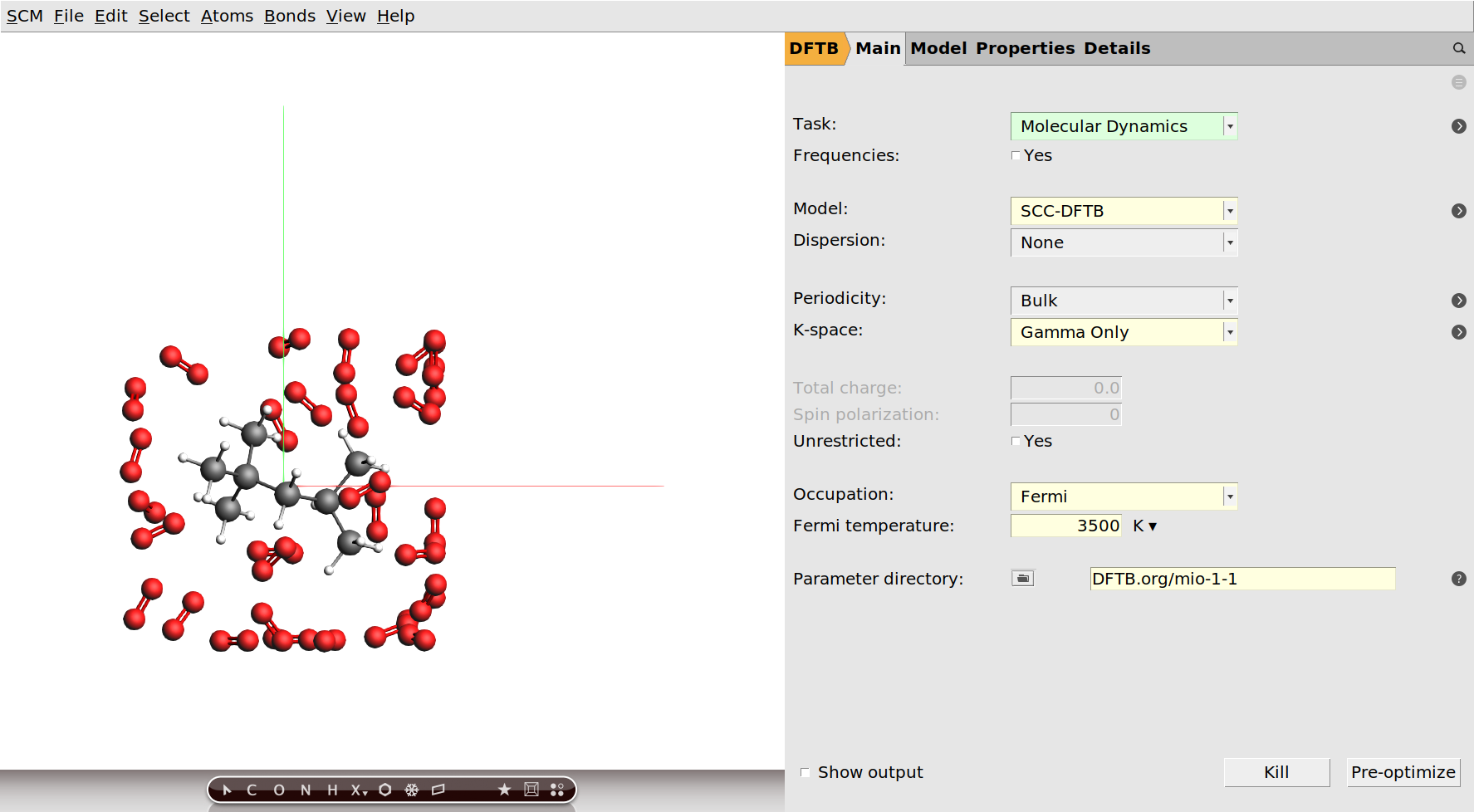
2. Set Periodicity → Bulk.

3. Select Occupation → Fermi and set the Fermi temperature to 3500K.

4. Set the Model to SCC-DFTB.

5. Set the Parameter directory to DFTB.org/mio-1-1.

6. Set K-space to Gamma Only.

Note

With the DFTB engine the calculation should take around two hours on a normal desktop computer. DFTB is a computationally efficient approximation to density functional theory (DFT), and generally quite accurate. If you want a faster calculation, you can alternatively run this tutorial with the ReaxFF engine. We suggest that you use the CHO.f parameters in this case.

Finally we need to specify that we want to run a molecular dynamics calculation and configure its details. We are going to run this calculation at the unrealistically high temperature of 3500K. For the purpose of this tutorial this is fine, as it means we can see an almost complete combustion happening within a couple of picoseconds.

: 1. Select Task → Molecular Dynamics.

2. Click on to go to the Model → MD panel.

3. Configure 10000 steps with a time step of 0.5fs. This will result in a 5ps long trajectory.

4. Set the sample frequency to 5. With a total of 10000 steps this will result in 2000 recorded samples.

5. Set the Initial temperature to 3500K.

We have set an initial temperature of 3500K, but in order to maintain this temperature throughout the simulation we should also attach a thermostat to our system. We will be using the Nosé–Hoover thermostat which yields good overall sampling results in general. The Nosé–Hoover damping constant is dependent on the system size because ideally it should match the period of the internal oscillations of the system. In the present case we use a reasonable value of 100fs, but one might want to test different values in a realistic setup.

: 1. Click on next to Thermostat to go to the Model → Thermostat panel.

2. Click the + button to add a thermostat to the simulation.

3. Select Thermostat → NHC (Nosé–Hoover chain).

4. Set 100fs as the damping constant.

5. Set 3500K as the Temperature.

Viewing the results¶

This is all the setup we need. We are now ready to run the calculation. While it is running, we can already follow its progress in AMSmovie.

: 1. Use the File → Run command.

2. When asked to save your input, save it with a name of your choice.

3. The AMSjobs window comes to the front and your job starts running.

4. Select your job and click SCM → Movie.

Depending on your initial conditions (and luck) it might take a while before the combustion starts and the isooctane disintegrates.

: 1. Leave the calculation running for at least half an hour.

When we set up the geometry of our system in AMSinput, we already saw bonds displayed between the atoms where we would expect bonds. These bonds were guessed by the GUI, which generally works well for isolated molecules around their equilibrium structures. However, the bonds you see while following your calculation in AMSmovie are actually calculated by the engine: In case of the DFTB engine this means that a Mayer bond order analysis based on the obtained electron density is performed at every frame of your MD calculation. (If you chose earlier to use the ReaxFF engine instead, you will see the bond orders that are used in the force field.)

Based on the bond orders calculated by the engine, the AMS driver will perform a molecule analysis for every frame of the trajectory. This basically detects which molecules we have in our system. This information can be visualized from AMSmovie. We can for example use it to not show all the oxygen molecules, since they are not really interesting and just block our view onto the isooctane we want to see.

: 1. Click MD Properties → Molecules.

2. Untick the box in the Show column for O2.

In the beginning we only have 30 O₂ molecules and the single isooctane (C₈H₁₈). As the reaction starts you will see intermediates and ultimately water and carbon dioxide. The 5ps trajectory we ran is probably not long enough to see a complete combustion, but you should already see some H₂O and CO₂ towards the end of your simulation.

Note

The list of detected molecules in the Molecules window does not update automatically while the calculation is still running. Close and reopen the window to see the latest molecules that have just formed.

For systems with periodic boundary conditions it can be a bit confusing to see atoms leave the box on one side and reappear on the other. For a better visualization we suggest that you make a few changes to the AMSmovie viewport on the left.

: 1. Enable showing the unit cell as a box by clicking View → Periodic → Show Unit Cell.

2. Show periodic images of all atoms by clicking View → Periodic → Repeat Unit Cells.

3. Adjust the transparency of the periodic images using the hotkeys Ctrl + j/n or via the View → Periodic → Transparency Periodic Cells menu.

This should give you a much clearer visualization:

You can download the movie here if it does not play in your browser.

Note

The results of the bond order analysis are real numbers and the bonds are simply drawn based on intervals for these bond orders, e.g. a single bond is shown if the calculated bond order is between 0.6 and 1.2. As such the bond visualization and also the molecule detection should be taken with a grain of salt, especially as molecules get close and interact with each other. You might for example see that two oxygen molecules that randomly approach each other quickly might be shown to be bonded (probably with dashed half-bonds) and momentarily be detected as an O₄ molecule.

You can also plot the number of molecules of a particular species by ticking the respective box in the Graph column of the Molecules window.

: 1. Let the calculation finish. This might take around two hours.

2. Click MD Properties → Molecules to open the Molecules window.

3. Tick the boxes in the Graphs column for O2, H2O and CO2.

As expected we see the consumption of oxygen and production of water and carbon dioxide. Furthermore we see the system’s potential energy go down, as the combustion releases energy.