Energy Decomposition Analysis (EDA)

• EDA with restricted fragments (ammonia borane)
• EDA with unrestricted fragments (ethane)
• EDA-NOCV: natural orbitals for chemical valence (metal complexes)

EDA with restricted fragments

This tutorial explains how to perform an energy decomposition analysis (EDA) [1] of ammonia borane, in which ammonia and borane have a donor-acceptor interaction with each other. In this way, you can examine which interactions result in a stable complex.

The bond energy (or binding energy) of H₃N-BH₃ is defined as:

\[\Delta E = E_{\text{H}_3\text{N}-\text{BH}_3} - E_{\text{NH}_3} -E_{\text{BH}_3}\]

in which E_NH3 and E_BH3 are the energies of the optimized reactants, and E_H3N-BH3 is the energy of the optimized complex.

Note

If you simply optimize a H₃N-BH₃ complex with ADF, the printed bond energy is not calculated from the above equation. Instead, it is calculated with respect to spherically symmetric spin-restricted atomic fragments. See more below.

The bond energy consists of the preparation energy (or strain energy, deformation energy), and the interaction energy:

\[\Delta E = \Delta E_{\text{prep}} + \Delta E_{\text{int}}\]

The preparation energy is the amount of energy that is required to deform the NH₃ and BH₃ from their equilibrium structure to the geometry they have in the complex. The interaction energy is the change in energy when the prepared fragments (NH₃ and BH₃ in the complex geometry) are combined to form the complex. A quantitative energy decomposition analysis (EDA) divides the interaction energy in the electrostatic interaction, Pauli repulsion, and attractive orbital interactions (oi):

\[\Delta E_{\text{int}} = \Delta V_{\text{elstat}} + \Delta E_{\text{Pauli}} + \Delta E_{\text{oi}}\]

The electrostatic interaction, which is usually attractive, is the energy between the unperturbed charge distributions of the prepared fragments. The Pauli repulsion is responsible for steric repulsion, it consists of the destabilizing interactions between occupied orbitals of the fragments. The orbital interaction accounts for charge transfer and polarization.

Geometry Optimizations of NH₃, BH₃ and H₃N-BH₃

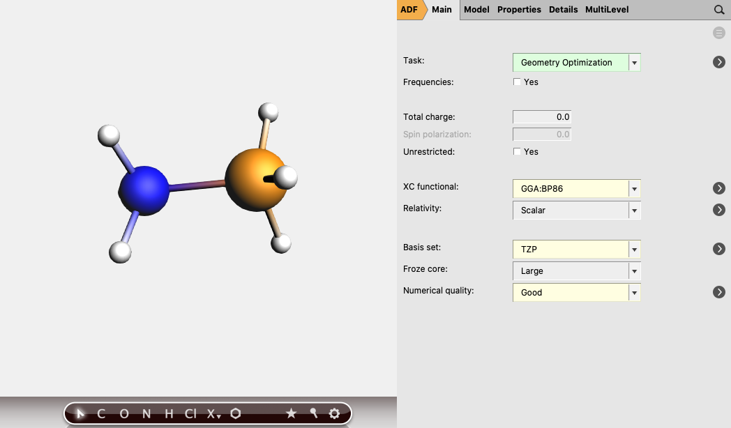
To calculate \(\Delta E\), the energies of optimized NH₃, BH₃ and H₃N-BH₃ need to be calculated. Note that another basis set and functional can be used as well. Symmetry will be used, which may help in the analysis. Open AMSinput (SCM → New Input), and perform the following steps:

1. Create NH₃: search for ammonia, click H3N: Ammonia (ADF)

2. Symmetrize the system by clicking on

3. Select Task → Geometry Optimization

4. Select XC functional → GGA:BP86

5. Select Basis set → TZP

5. Select Numerical quality → Good

7. Run the calculation with File → Run (save with the name ammonia)

Repeat the above steps for BH₃:

Create BH₃: → Metal Complexes → ML3 Trigonal Planar.

Select the central atom, Atoms → Change Atom Type to B, then change the three “ligands” to H.

Repeat steps 2-7 above (save with the name borane).

Repeat the above steps for H₃N-BH₃.

To create H₃N-BH₃, combine the previous two systems by copying and pasting.

Repeat steps 2-7 (save with the name ammoniaborane).

EDA: single-point calculation with molecular fragments

When the H₃N-BH₃ calculation has finished, AMSinput will ask whether to update the coordinates.

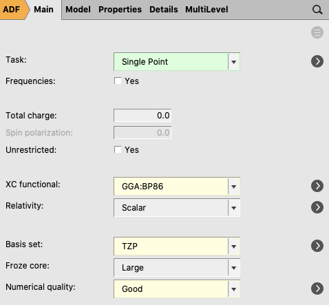
1. Select Yes → New Job, or manually create a new job with the optimized geometry and the previous calculation settings (XC functional, basis set, numerical quality).

2. Set Task → Single Point.

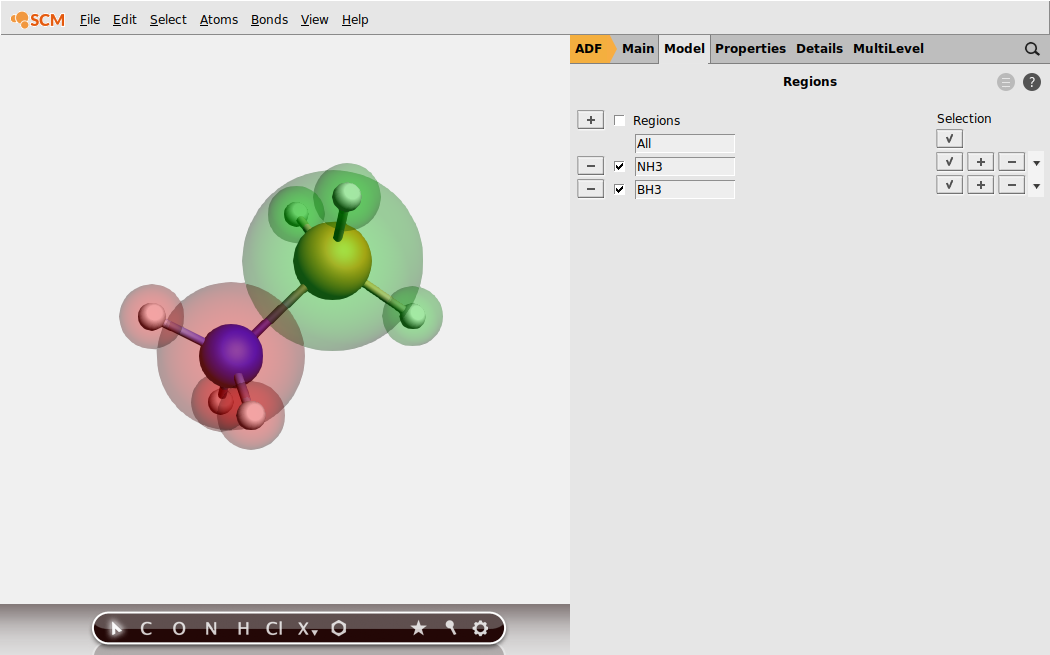
3. Go in the panel bar to Model → Regions

4. Select the atoms of NH₃ and click the button next to Regions, and rename Region_1 to NH3

5. Select the atoms of BH₃ and click also on the button, and rename Region_2 to BH3.

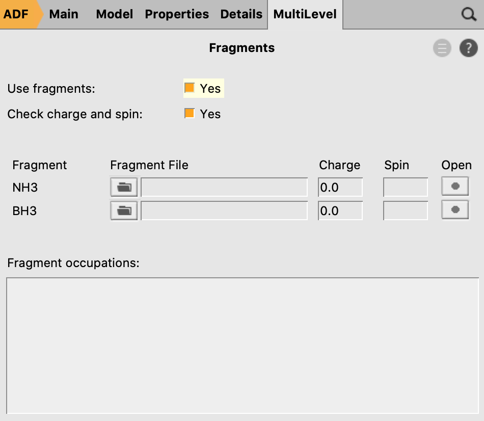
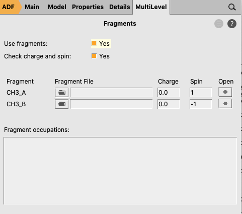
6. Go in the panel bar to MultiLevel → Fragments

7. Check the ‘Use fragments’ check box

8. Run the calculation (save with the name EDA_ammoniaborane).

The job actually runs three separate calculations. First, single point calculations of NH₃ and BH₃ in their prepared geometry are run. The adf.rkf files of those single point computations are then used for the fragment analysis.

Bond energy, preparation energy, interaction energy

The energy of a calculation can be found at the bottom of the logfile (SCM → Logfile), in the output (SCM → Output), or in the binary output file (SCM → KFbrowser).

To tabulate the energies from all previous calculations, either

• use one of the above methods to get the energy for each calculation
• Build a spreadsheet summary: In AMSjobs (SCM → Jobs), select the ammonia, borane, ammoniaborane, EDA_ammoniaborane, EDA_ammoniaborane.NH3, and EDA_ammoniaborane.BH3 jobs by holding Ctrl and clicking on them. Then go to Tools → Build spreadsheet, set the Energy unit to kcal/mol, and click Do It. Save with the name report.xlsx.

Fig. 36 Spreadsheet summary of all calculations. The “Notes” and energy calculations were manually added.

\[\Delta E = E_{\text{H}_3\text{N}-\text{BH}_3} - E_{\text{NH}_3} -E_{\text{BH}_3}\]

The bond energy \(\Delta E\) of H₃N-BH₃ was calculated to be -31.81 kcal/mol with these settings. (-838.47 - (-444.53) - (-362.14) = -31.81)

The preparation energy for BH₃ (12.64 kcal/mol, calculated as -349.50-(-362.14)) is much larger than that for NH₃ (0.11 kcal/mol). This is because the structure of the fully relaxed NH₃ is only slightly different from the structure of the NH₃ fragment in H₃N-BH₃. However, the structure of the fully relaxed flat BH₃ (symmetry D_3h) is substantially different than the structure of the BH₃ trigonal pyramidal fragment in H₃N-BH₃ (symmetry C_3v):

The interaction energy is simply the “bond energy” output by ADF for the EDA_ammoniaborane job. This is because that job used the reactants in the prepared geometries as fragments.

EDA Analysis

The energy decomposition of the interaction energy of H₃N-BH₃ can be found in the output file of the fragment analysis (job ammoniaborane, SCM → Output, followed by Properties → Bonding Energy Decomposition). You can find for instance that H₃N-BH₃ has an interaction energy of -44.55 kcal/mol, which consists of a Pauli repulsion of 107.97 kcal/mol, an electrostatic interaction of -77.44 kcal/mol, and an orbital interaction of -75.09 kcal/mol.

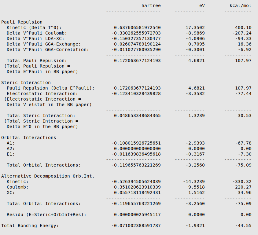
The orbital interaction is decomposed into contributions from different irreducible representations of the molecular point group. In this case the contributions from A1 (\(\sigma, \sigma^*\)-orbitals) are much more important than those from E1 (\(\pi, \pi^*\)-orbitals).

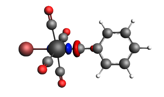
With AMSlevels the molecular orbital diagram can be visualized, in which one can see a donor-acceptor interaction and (repulsive) interactions between occupied orbitals.

1. SCM → Levels

2. In AMSlevels, click on View → Labels → Show

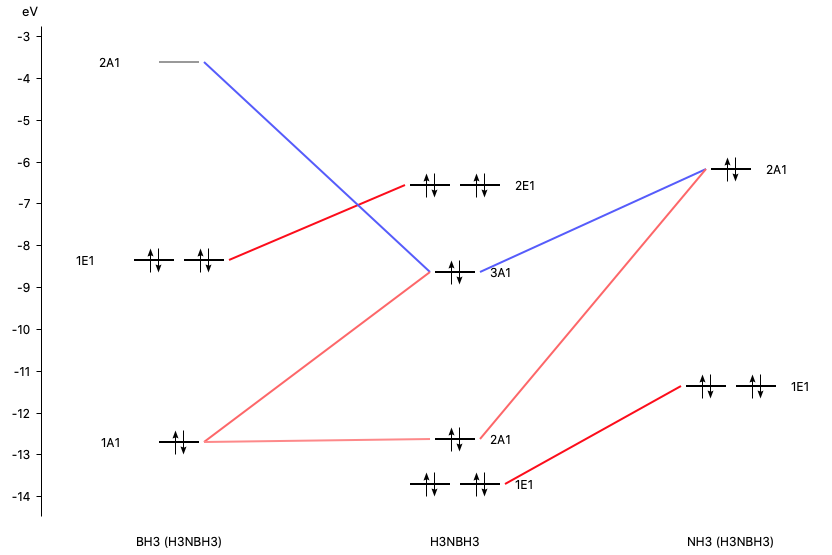
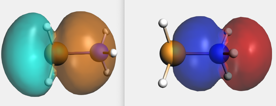
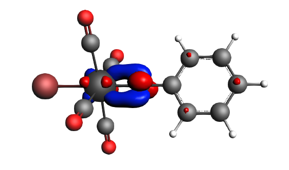
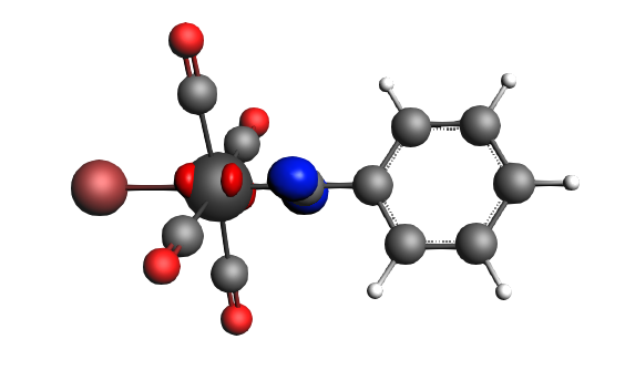
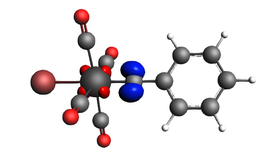
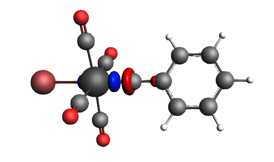
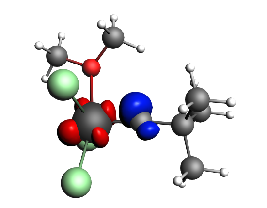
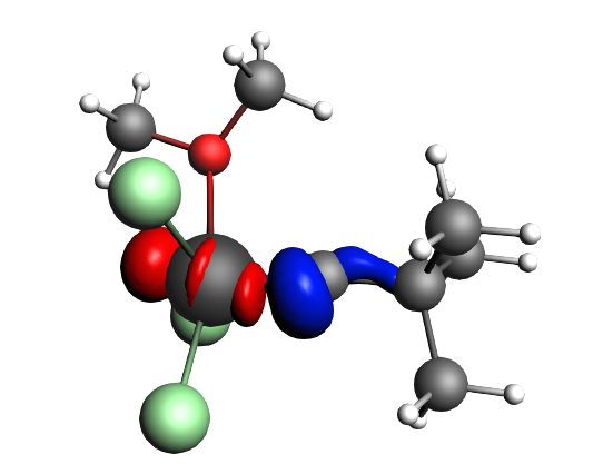
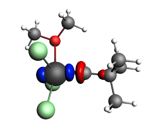
By right-clicking the BH₃ 2A1 fragment orbital (LUMO of BH₃, acceptor orbital) you can select the corresponding SFO (symmetrized fragment orbital), which can be visualized with AMSview. Similarly, you can select the NH₃ 2A1 fragment orbital (HOMO of NH₃, donor orbital). After some manipulations, using 50% opacity, you can get the following two AMSview windows that show these fragment orbitals.

EDA with unrestricted fragments

This tutorial explains how to perform an energy decomposition analysis (EDA) of a molecule with unrestricted fragments, for example the CH₃ groups of ethane. Hereby, the user can examine which interactions result in the stable molecule. To see an explanation of these different interactions or to do an EDA without unrestricted fragments, see the EDA of Ammonia Borane tutorial.

Geometry Optimization

The geometry of the reactants and the product (complex) must be optimized. Note that another basis set and functional can be used as well. Symmetry will be used, which may help in the analysis.

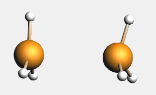
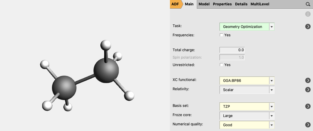
For ethane:

1. In AMSinput make the structure or search for the structure in the search box in the panel bar

2. Symmetrize the system by clicking on

3. Select Task → Geometry Optimization

4. Select XC functional → GGA:BP86

5. Select Basis set → TZP

5. Select Numerical quality → Good

7. Run the calculation with File → Run (give an appropriate name to your calculations)

8. When the run has finished, click ‘Yes’ to import the optimized coordinates and save it

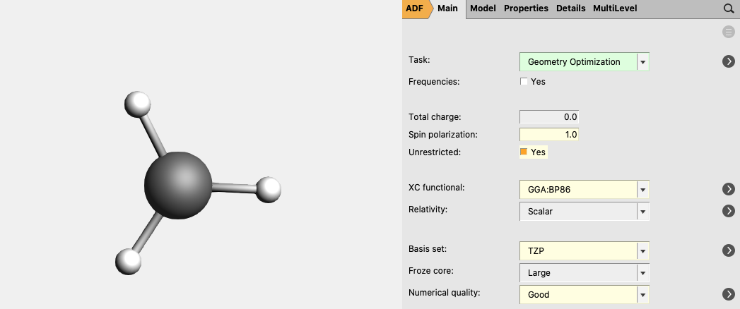
For CH₃ (methyl) an unrestricted calculation is needed:

1. In AMSinput make the structure or search for the structure in the search box in the panel bar

2. Symmetrize the system by clicking on

3. Select Task → Geometry Optimization

4. Check the Unrestricted box.

5. Enter 1.0 as Spin polarization

6. Select XC functional → GGA:BP86

7. Select Basis set → TZP

8. Select Numerical quality → Good

9. Run the calculation with File → Run (give an appropriate name to your calculations)

10. When the run has finished, click ‘Yes’ to import the optimized coordinates and save it

The bond energy of C₂H₆ can be calculated by subtracting the energies of the reactants (two CH₃) from the energy of the complex. The energies can be found at the bottom of the logfile or in the output.

\[\Delta E = E_{C_2H_6} - 2 E_{CH_3}\]

The bond energy of C₂H₆ was calculated to be -93.53 kcal/mol with these settings. (-920.23 - 2*(-413.35)) = -93.53)

EDA

Single point calculations of the CH₃ groups in the geometry they have in the product are needed to perform an EDA. Note that one sometimes need to change the electron configuration of the fragments to make them so called ‘prepared for bonding’ in order to minimize the Pauli repulsion in the electron pair bond. This is not needed in this simple example.

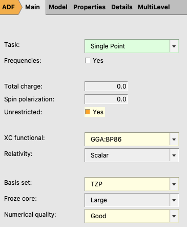
1. Perform a new calculation with the optimized molecule, ethane

2. Select the Task Single Point

3. Check the Unrestricted box.

4. Select XC functional → GGA:BP86

5. Select Basis set → TZP

6. Select Numerical quality → Good

7. Go in the panel bar to Model → Regions

8. Select the atoms of one CH₃ group and click the button next to Regions

9. Select the atoms of the other CH₃ group and click also on the button

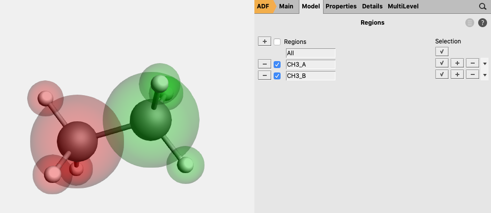
10. Go in the panel bar to MultiLevel → Fragments

11. Check the ‘Use fragments’ check box (A warning will popup regarding NOSYM symmetry)

12. Enter as spin polarization 1 for one of the fragments and -1 for the other fragment

The symmetry has been adjusted to NOSYM. However, we want to use symmetry. Besides setting the symmetry to AUTO, in this case we also need to symmetrize the coordinates again, since using fragments will lower the symmetry of ethane that ADF can use from D_3d to C_3v. Note that in this case the symmetrization will only reorient the geometry in order to fulfill the molecular orientation requirements in ADF such that ADF can use symmetry.

13. Go in the panel bar to Details → Symmetry

14. Select Symmetry → AUTO

15. Symmetrize the system by clicking on

16. Save it and run the calculation

Analysis

The different energies, where the interaction energy of the CH₃ groups of ethane consists of, are noted in the output (Properties → Bonding Energy Decomposition). It can be noticed that the interaction energy of -111.41 kcal/mol is build out of 180.02 kcal/mol Pauli repulsion, -125.43 kcal/mol electrostatic interaction, and -166.02 kcal/mol orbital interactions.

The orbital interaction is decomposed into contributions from different irreducible representations of the molecular point group. In this case the contributions from A1 (\(\sigma, \sigma^*\)-orbitals) are much more important than those from E1 (\(\pi, \pi^*\)-orbitals).

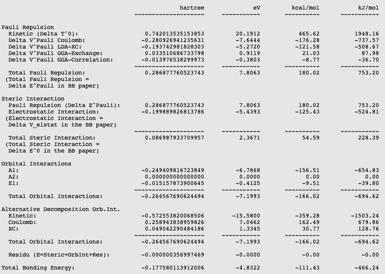
The bond energy was calculated previously to be -93.53 kcal/mol and accordingly the preparation energy can be calculated to be 17.88 kcal/mol (=-93.53-(-111.41)). The preparation energy for one CH₃ fragment is 8.95 kcal/mol, the difference between the bond energy of the CH₃ trigonal pyramidal fragment (-404.40 kcal/mol) and the fully relaxed planar CH₃ molecule (-413.35 kcal/mol). The preparation energy of the other CH₃ fragment is the same. Note that the energies of the fragments can be found at the bottom of the logfile or in the output of the fragments.

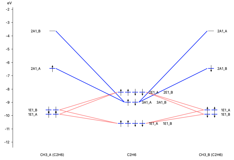
With AMSlevels the molecular orbital diagram can be visualized, in which one can see an electron-pair bond and (repulsive) interactions between occupied levels.

Dispersion correction

Dispersion energy can be of importance in complexes with weak bonds. The dispersion energy is a long-ranged electron correlation effect. When using, for example, a DFT-D3 functional or a DFT-D4 functional the dispersion corrected energy will also be a part of the interaction energy:

\[\Delta E_{int} = \Delta V_{elstat} + \Delta E_{Pauli} + \Delta E_{oi} + \Delta E_{disp}\]

The dispersion corrected interaction energy will be printed in the output file just as the electrostatic interaction, Pauli repulsion, and orbital interactions. The dispersion corrections are XC functional dependent, and contain fitted parameters. For many XC functionals such parameters are available in AMS.

EDA-NOCV: natural orbitals for chemical valence

An energy decomposition analysis - natural orbitals for chemical valence (EDA-NOCV), also known as extended transition state - natural orbitals for chemical valence (ETS-NOCV), can be used for the analyzation of [TM]-L bonds in transition metal compounds. This method combines the energy decomposition analysis [1] with the natural orbitals for chemical valence [2]. This tutorial will show how to use the EDA-NOCV method for a Fischer-type carbyne complex and a Schrock-type carbyne complex, based on the paper of Jerabek et al. [3]

The EDA-NOCV/ETS-NOCV method gives insight in the orbital interactions for non-symmetric molecules, because the deformation density is decomposed into different components (σ, π, δ) of the chemical bond. In the ETS-NOCV: Natural Orbitals for Chemical Valence documentation more information about this method can be found.

In carbyne complexes, various types of orbital interaction between a ligand and the TM can be distinguished:

• donor–acceptor complexes possessing dative bonds (Fischer‐type carbynes)
• electron‐sharing bonds (Schrock‐type carbynes)

Here we follow Ref. [3], in order to see whether the results of the EDA-NOCV calculations may provide a useful classification of the TM compounds into the these two types of molecules. Note that this example focuses on the understanding of [TM]-L bonds and compares results using different electron configurations of the fragments. This example does not calculate bond energies.

Some remarks on the analysis. The EDA depends on the fragments chosen, whether neutral or charged fragments are used, and which spin state they have. For the EDA-NOCV method it is necessary that the sum of the number of spin-α orbitals in the fragments is the same as in number of spin-α orbitals the full complex, likewise for the number of spin-β orbitals. If there is (near) degeneracy between different electron configurations of the fragments, for the analysis it is best to use the electron configuration of the fragments such that they are so called ‘prepared for bonding’ in order to minimize the Pauli repulsion in the electron pair bond. For example, if one has two fragments which both have unpaired electrons, one typically would put the unpaired electrons of the first fragment in the spin-α orbitals and the unpaired electrons of the second fragment in the spin-β orbitals. In this example this will be used, but not all possible reasonable electron configurations will be investigated, which might have been better ‘prepared for bonding’. Note that here so called ‘real’ unrestricted fragments will be used, which was not possible in the ADF version that was used in Ref. [3]. This means that the energies in the EDA that will be reported here are not directly quantitatively comparable to those in Ref. [3].

An EDA-NOCV will be performed on the Fischer-type carbyne complex Br(CO)₄W-CPh and on the Schrock-type carbyne complex Cl₃(dme)W-CCMe₃ with fragments in 1. the singlet state (dative bonding), 2. the quartet state (electron-sharing bonding), and 3. the doublet state (mixed dative/electron-sharing bonding). The geometry of Br(CO)₄W-CPh can be downloaded here and the geometry of Cl₃(dme)W-CCMe₃ can be downloaded here. Single Point calculations will be performed on these optimized complexes.

1. Dative bonding

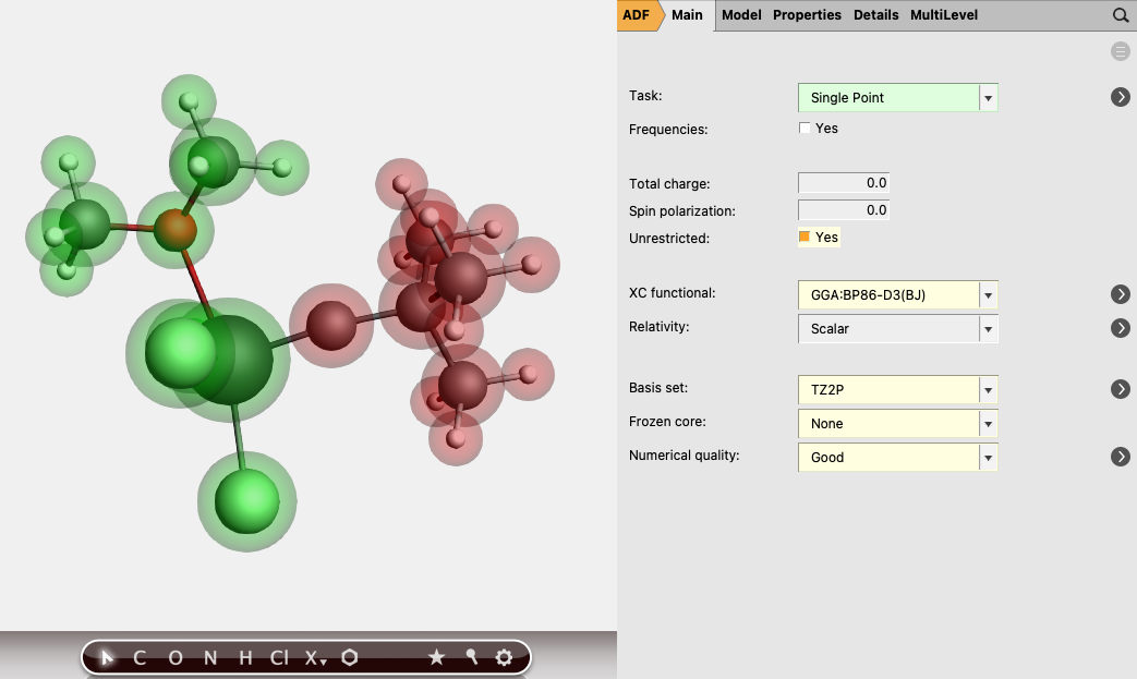
These calculations are based on the paper of Jerabek et al. [3] and therefore the following level of theory is used. Perform the following steps for the Br(CO)₄W-CPh and Cl₃(dme)W-CCMe₃ complexes you just downloaded:

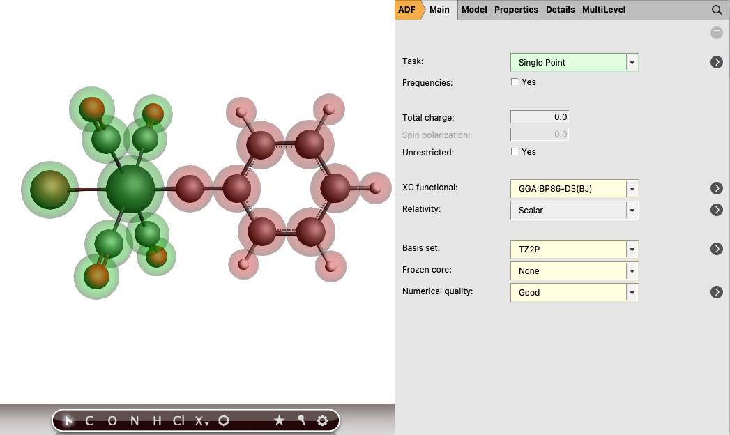
1. Open the geometry of the complex in AMSinput

2. Make sure that the Task is set at Single Point

3. Select the GGA:BP86-D3(BJ) XC functional and TZ2P Basis set

4. Make sure that the Relativity is set at Scalar

5. Select Frozen Core → None and Numerical quality → Good

6. Go in the panel bar to Model → Regions

7. Select the atoms of the ligand (C-tBu or C-Ph group) and click the button next to Regions

8. Select all other atoms of the complex (by Select → Invert Selection) and click the button again

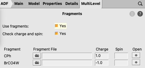
9. Go in the panel bar to MultiLevel → Fragments

10. Tick the Use fragments box (the Check charge and spin box and no symmetry will be set)

11. Enter as charge for the ligand fragment 1.0 and for the other fragment -1.0

13. Go in the panel bar to Properties → ETS-NOCV

14. Select an Closed-Shell ETS-NOCV analysis

15. Run the calculation

Note that one may have SCF problems for the fragment [Cl₃(dme)W]^-1

In this case both charged fragments are calculated in the singlet state.

SCF problems

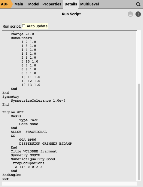
The fragment [Cl₃(dme)W]^-1 has problems with SCF convergence. It is difficult (or impossible) to converge the SCF with an aufbau solution. Therefore one can use an explicit non-aufbau electron configuration. Note that the following is an expert option. If you do not include the next expert steps you may get a different non-aufbau solution, and thus a different energy decomposition analysis for Cl₃(dme)W-CCMe₃ for this case of charged fragments.

Relevant only for the fragment [Cl₃(dme)W]^-1 of Cl₃(dme)W-CCMe₃

Open the fragment [Cl₃(dme)W]^-1 AMSinput

Go in the panel bar to Details → Run Script

Enter in Engine ADF part:

IrrepOccupations

A 148 0 0 2 2

End

Select File → Save

Close the fragment [Cl₃(dme)W]^-1 AMSinput

Open the Cl₃(dme)W-CCMe₃ AMSinput

Run the calculation

2. Electron-sharing bonding

To analyse the electron-sharing bonding of [TM]-L, step 1-8 must be performed again. After that, the following steps can be made:

9. In the Main panel bar tick the box for an Unrestricted calculation

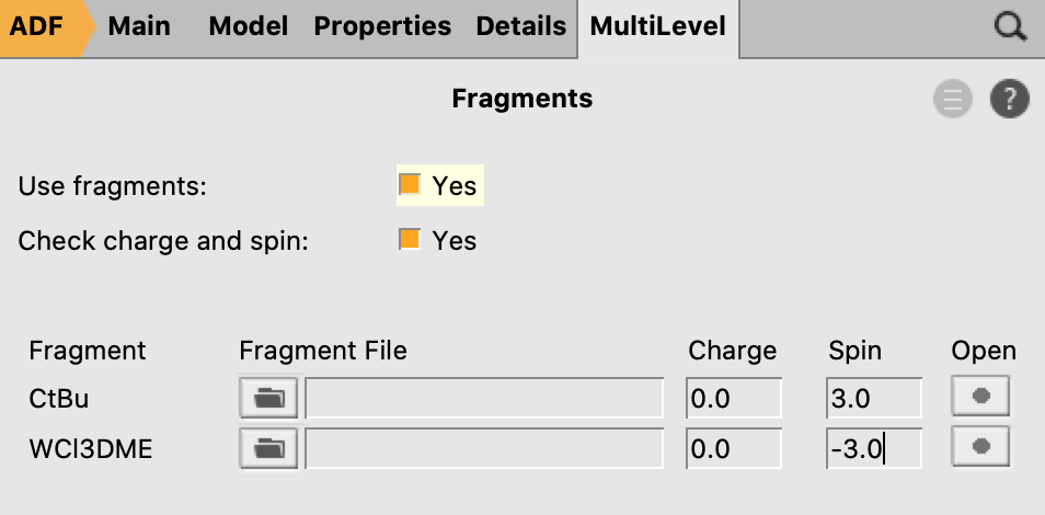
10. Go in the panel bar to MultiLevel → Fragments

11. Tick the Use fragments box (the Check charge and spin box and no symmetry will be set)

12. Enter as spin polarization for the ligand fragment 3.0 and for the other fragment -3.0 (the charges should be set to 0 for both fragments).

13. Go in the panel bar to Properties → ETS-NOCV

14. Select an Open-Shell ETS-NOCV analysis

15. Run the calculation

In this case both neutral fragments are calculated in the quartet state (more precisely they have |S_z|=3/2).

3. Dative/Electron‐sharing bonding

To analyse the mixed dative/electron‐sharing bonding of [TM]-L, the steps for the electron-sharing must be performed again, apart from step 12, which should be

12. In the panel bar MultiLevel → Fragments enter as spin polarization for the ligand fragment 1.0 and for the other fragment -1.0 (the charges should be set to 0 for both fragments).

such that both neutral fragments are calculated in the doublet state (more precisely they have |S_z|=1/2). Note that the fragment CCMe₃ has near degenerate solutions in case it is calculated in the doublet state, and that one solution may have a corresponding electron configuration that may be better ‘prepared for bonding’ than another. This will not be investigated further.

EDA

The different energy terms of the interaction between the ligand and its transitions state complex are noted in the output (Properties → Bonding Energy Decomposition). The following energy terms will be found for Br(CO)₄W-CPh and Cl₃(dme)W-CCMe₃ (in kcal/mol):

Br(CO) 4 W-CPh	Dative	Electron-sharing	Dative/Electron‐sharing
ΔEint	-261.9	-191.0	-154.8
ΔEPauli	232.8	230.3	292.5
ΔVelstat	-211.0	-173.3	-214.7
ΔEoi	-275.3	-239.6	-224.3
ΔEdisp	-8.4	-8.4	-8.4

Cl 3 (dme)W-CCMe 3	Dative	Electron-sharing	Dative/Electron‐sharing
ΔEint	-427.4	-194.7	-177.1
ΔEPauli	303.4	302.2	690.4
ΔVelstat	-251.2	-224.4	-436.2
ΔEoi	-468.6	-261.3	-420.1
ΔEdisp	-11.2	-11.2	-11.2

The method which results in an orbital interaction closer to zero gives the commonly accepted chemical interpretation (dative or electron-sharing), see Ref. [3].

For the Fischer-type carbyne complex Br(CO)₄W-CPh the orbital interaction is closer to zero for the dative/electron sharing bonding with an orbital interaction of -224.3 kcal/mol (vs -239.6 or -275.3 kcal/mol).

For the Schrock-type carbyne complex Cl₃(dme)W-CCMe₃ the orbital interaction is closer to zero for the electron-sharing bonding with an orbital interaction of -261.3 kcal/mol (vs -420.1 or -468.6 kcal/mol).

EDA-NOCV Fischer‐type carbyne complex

The best description for the Fischer‐type carbyne complex Br(CO)₄W-CPh is found for neutral fragments in their electronic doublet state (|S_z|=1/2), which engage in a mixture of dative bonding (σ donation and π backdonation) and one electron‐sharing π bond, as can be seen in the next NOCV analysis.

Go to AMSjobs

Select the Br(CO)₄W-CPh job with neutral fragments in their electronic doublet state (the third job, dative/electron-sharing bonding)

Open AMSview (SCM → View)

Select Fields → Grid → Medium)

Select Add → Isosurface: With Phase)

In the field select menu on the bottom: select NOCV Def Densities…

Select NOCV_Def_Density with largest eigenvalue

Change isosurface value to 0.01

Repeat this for NOCV_Def_Density with the 5 highest eigenvalues

The direction of the charge flow from fragments to full complex in the next pictures is from red → blue. The orbital interaction energy contributions from each NOCV pair can be found in the output (Properties → ETS - NOCV).

α-Δρ ΔE=-80 kcal/mol (|v|=1.00), electron‐sharing π bond

left: β-Δρ ΔE=-30 kcal/mol (|v|=0.54), right: β-Δρ ΔE=-39 kcal/mol (|v|=0.53), π backdonation

left: β-Δρ ΔE=-30 kcal/mol (|v|=0.34), right: α-Δρ ΔE=-29 kcal/mol (|v|=0.34), σ donation

EDA-NOCV Schrock‐type carbyne complex

The best description for the Schrock‐type carbyne complex Cl₃(dme)W-CCMe₃ is found for neutral fragments in their electronic quartet state ((|S_z|=3/2), which engage in one electron-sharing σ bond and two electron‐sharing π bonds, as can be seen in the next NOCV analysis.

Go to AMSjobs

Select the Cl₃(dme)W-CCMe₃ job with neutral fragments in their electronic quartet state (the second job, electron-sharing bonding)

Open AMSview (SCM → View)

Select Fields → Grid → Medium

Select Add → Isosurface: With Phase

In the field select menu on the bottom: select NOCV Def Densities…

Select NOCV_Def_Density with largest eigenvalue

Change isosurface value to 0.01

Repeat this for NOCV_Def_Density with the 6 highest eigenvalues

The direction of the charge flow from fragments to full complex in the next pictures is from red → blue. The orbital interaction energy contributions from each NOCV pair can be found in the output (Properties → ETS - NOCV).

top-left: α-Δρ ΔE=-32 kcal/mol (|v|=0.65), top-right: β-Δρ ΔE=-37 kcal/mol (|v|=0.65), bottom-left: α-Δρ ΔE=-30 kcal/mol (|v|=0.62), bottom-right: β-Δρ ΔE=-51 kcal/mol (|v|=0.55), two electron‐sharing π bonds

left: β-Δρ ΔE=-73 kcal/mol (|v|=0.54), right: α-Δρ ΔE=-33 kcal/mol (|v|=0.42), one electron-sharing σ bond

References

[1]	(1, 2) F.M. Bickelhaupt, E.J. Baerends, Kohn-Sham Density Functional Theory: Predicting and Understanding Chemistry, Reviews in Computational Chemistry 15, 1 (2000)

[2]	M. Mitoraj, A. Michalak, Donor–Acceptor Properties of Ligands from the Natural Orbitals for Chemical Valence Organometallics 26, 6576 (2007)

[3]	(1, 2, 3, 4, 5, 6) P. Jerabek, P. Schwerdtfeger, G. Frenking, Dative and Electron-Sharing Bonding in Transition Metal Compounds Journal of Computational Chemistry 40, 247 (2019)