Polymers¶

Method 1: Using ADF¶

This is the standard method for using compounds not already present in the database. This method requires an ADF and COSMO calculation, but polymer calculations can require a lot of atoms, sometimes making these calculations expensive. For this method, we must first perform a geometry optimization and then a single point COSMO calculation. The required steps for this calculation are as follows:

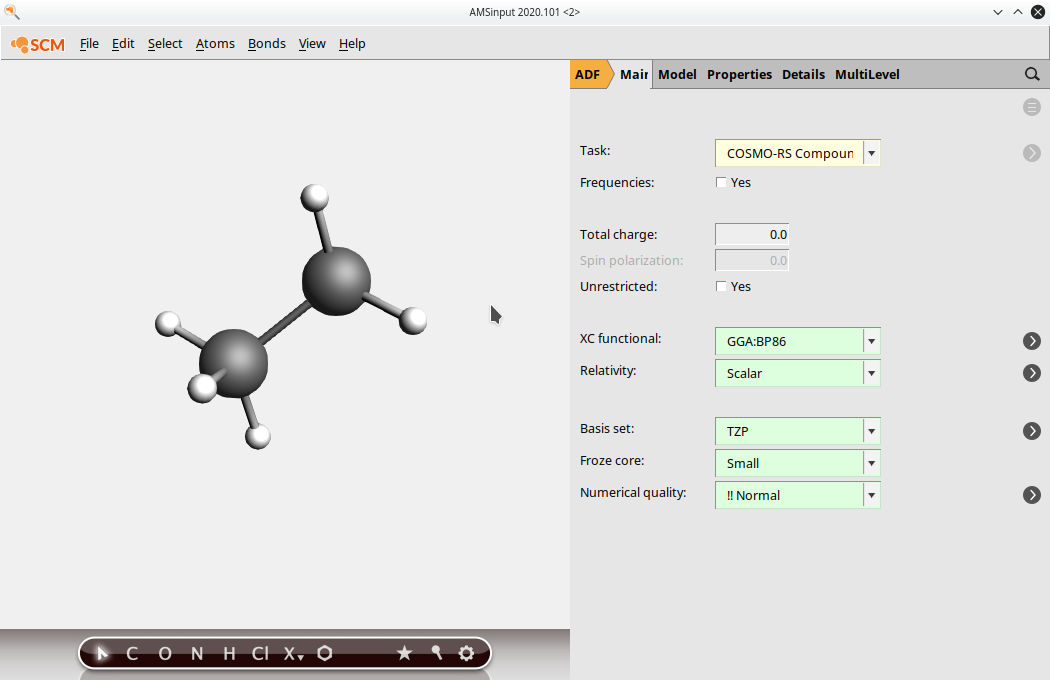
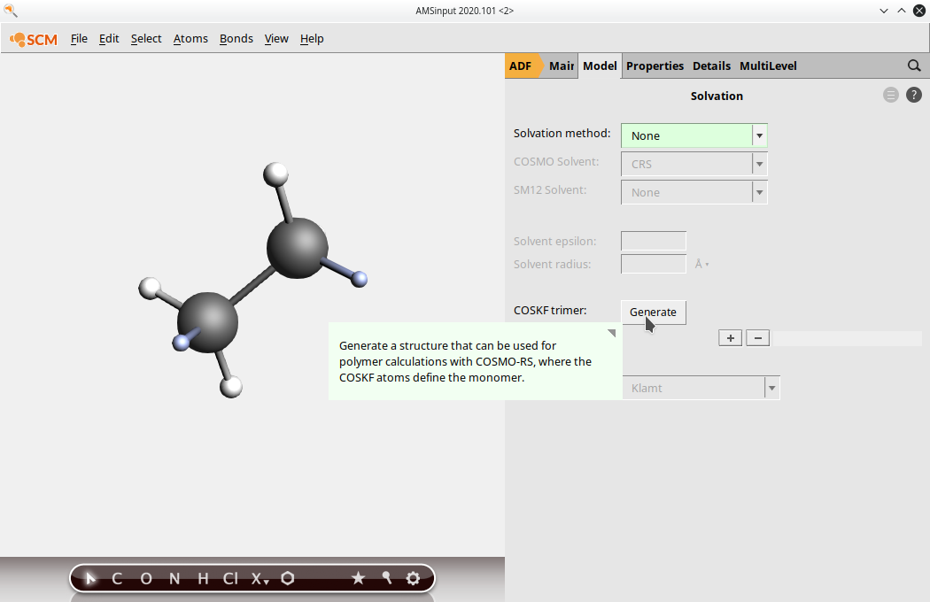
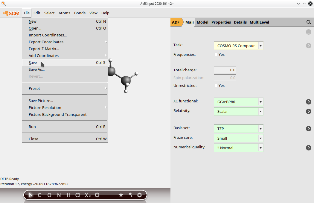
Start AMSinput (SCM → New Input)

Select Task → COSMO-RS Compound

Input the structure of a single monomer unit of your polymer

Add dummy (“Xx”) atoms corresponding to where the monomer is attached to other monomers in the polymeric structure

Go to Model → Solvation

click “Generate” next to “COSKF trimer”

Save/run your input file

We will illustrate the process of new polymer input using polyethylene below:

(1) Select Task → COSMO-RS Compound, Input the monomer structure

(2) Select the atoms that should be replaced by other monomer units in the full polymer. Note: depending on how you have inputted the structure, you may have to add these atoms. Be sure to check that all of the correct atoms are present. Select multiple atoms by holding the Shift key and clicking.

(3) Click on Atoms → Change Atom Type and replace the atoms with “Xx”

(4) Go to Model → Solvation and click “Generate” next to “COSKF trimer”

(4.5) (Optional, but recommended) Go to the DFTB menu, select GFN1-xTB in the Model field, and press the Pre-optimize button. This will provide a good initial geometry for the subsequent ADF calculation.

(5) Go back to the ADF panel and select Task: COSMO-RS Compound save your input file

(6) Run the job (File → Run). After running the job, open the newly created .coskf file in the COSMO-RS GUI. Note that depending on the order of opening GUI windows the .coskf file may already have been opened by the COSMOS-RS GUI. You can see the COSMO surface by first selecting your new compound on the Compounds → List of added compounds window. Then press the “Show 3D” button, which opens an AMSview window. From AMSview, click Add → COSMO: Surface Charge Density → On COSMO surface points. This could produce the image below:

Method 2: Using FastSigma to estimate a polymer’s sigma profile¶

Because ADF calculations for large polymers can be expensive, it is sometimes preferred to estimate the necessary parameters to perform a COSMO-RS calculation. This can be done with the FastSigma tool available from the GUI or the command line. To use this tool from the COSMO-RS GUI, use the following steps:

Select Compounds → List of added compounds

In the top left corner in the SMILES input field, type the CurlySMILES for polystyrene C{-}C{n+}(c1ccccc1)

Click Add and save the file

The above steps should involve the following (main) step:

Polymer/Average Molecular Weight¶

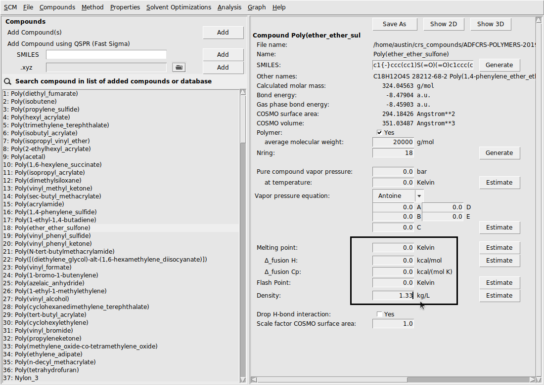
Because polymers of the same type can come in many lengths, it is important to be able to adjust the average molecular weight of a polymer. This is done from the compounds menu: Compounds → List of Added Compounds. Below, we show an example of setting the average molecular weight for Poly(ether_ether_sulfone) (PEES):

Additionally, to specify that a compound should be treated like a polymer, the Polymer box should be checked (shown in the image above). The number of repeat units will be set to the average molecular weight divided by the molar mass of the compound (the compound is assumed to the be monomer).

Density¶

Due to a modified combinatorial term for polymers, densities are required for every species in a calculation involving any polymers. In the ADFCRS database, many polymers already have a recommended density value, which should provide reasonable results under standard temperature and pressure conditions. However, it is well-known that for many polymers these density values can be sensitive to temperature and solvent. In these cases – or in cases where there is no recommended density value given – the density can be input from the compounds menu: Compounds → List of Added Compounds.

Here, we show an example of inputting the density for Poly(ether_ether_sulfone) (PEES):

Activity coefficients¶

For this calculation, we estimate the activity coefficients in a Poly(ethylene)/Benzene mixture. Because this is a calculation involving polymers, we will need the density of both Poly(ethylene) and Benzene. There is a recommended value of Poly(ethylene) given (0.852), so we can use that value. For Benzene, we’ll enter a value of 0.876. Use the following summary of steps to perform the calculation:

Compounds → List of Added Compounds

Select Benzene

Set Density to 0.876

Properties → Activity Coefficients

Select 2 Components

Select Mass fraction

Select Poly(ethylene) and Benzene

Set mass fraction of Poly(ethylene) to 0.5

Set mass fraction of Benzene to 0.5

Click Run

Click OK to the ‘Warning: no solutes found’

The result of this calculation is the following:

Notice that some non-standard properties are given: weight fraction activity coefficient (= mass fraction activity coefficient), volume fraction activity coefficient, and Flory-Huggins \(\chi\).

Vapor pressure of a mixture¶

Now, we will estimate the vapor pressure of a mixture of Poly(dimethylsiloxane), Methanol, and n-Hexane. Use the following summary of steps to perform the calculation:

Compounds → List of Added Compounds

Select Methanol

Set Density to 0.792

Click Estimate next to Vapor pressure equation

Select Hexane

Set Density to 0.655

Click Estimate next to Vapor pressure equation

Properties → Vapor pressure mixture

Select 3 Components

Select Mass fraction

Select Poly(dimethylsiloxane), Methanol, and Hexane

Set mass fraction of Poly(dimethylsiloxane) to 0.5

Set mass fraction of Methanol to 0.25

Set mass fraction of Hexane to 0.25

Adjust the temperature range from 298.15 K to 398.15 K

Click Run

The result of this calculation is the following:

Note that estimated properties are calculated with the Property estimation tools

Partition Coefficients (LogP)¶

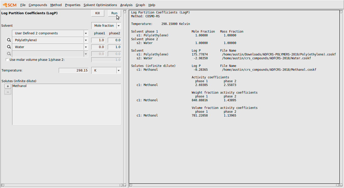
Now, we’ll calculate the partition coefficient of Methanol between a water and poly(ethylene) phase.

Compounds → List of Added Compounds

Select Methanol

Set Density to 0.792

Select Water

Set Density to 1.0

Properties → Partition Coefficients (LogP)

User Defined 2 components

Select Poly(ethylene) and Water

Set mole fraction Poly(ethylene) to 1.0 in phase 1

Set mole fraction Water to 1.0 in phase 2

Select Methanol in the Solutes (infinite dilute) box

Click Run

The output of this calculation is shown below:

Solubility in Pure Solvents¶

In this example, we’ll calculate the solubility of Hexane gas in Poly(styrene) over the temperature range 398.15 K to 498.15 K and over the pressure range 1.0 bar to 4.0 bar.

Compounds → List of Added Compounds

Select Hexane

Set Density to 0.655

Click Estimate next to Vapor pressure equation

Properties → Solubility in Pure Solvents

Select Poly(styrene) in Pure Compound Solvents

Select Hexane as the Solute

Select Gas for the solute type

Set the temperature range from 398.15 K to 498.15 K

Set the number of steps for pressure to 3

Set the pressure range from 1.0 bar to 4.0 bar

Click Run

Click Graph → Y axes → Solubilty (g/L solvent)

Binary Mixture and Flory-Huggins \(\chi\)¶

In this example, we will calculate binary mixture properties (including the \(\chi\)) over the entire range of compositions. We will do this for a binary mixture of Benzene and Poly(ethyl_ethylene) and use COSMO-SAC (the 2013-ADF Xiong parameters).

Compounds → List of Added Compounds

Select Benzene

Set Density to 0.876

Method → COSMO-SAC

Method → Parameters

Select the 2013-ADF Xiong parameters

Properties → Binary Mixture VLE/LLE

Select Poly(ethyl_ethylene) as Compound 1

Select Benzene as Compound 2

Select Mass Fraction

Click Run

Click Graph → X axes → w1: mass fraction 1

Click Graph → Y axes → Flory-Huggins 𝛘

The result of this calculation is the following: