Thermal expansion coefficients of thermoset polymers

In this ReaxFF tutorial thermal expansion coefficients, CTE, are calculated from a polymer’s strain vs. temperature dependence.

The systems and workflows presented here are originally described in the publication Effect of chemical structure on thermo-mechanical properties of epoxy polymers: Comparison of accelerated ReaxFF simulations and experiments, Polymer 159, 354-368 (2018).

The tutorial consists of the following steps:

• Importing the polymer structure
• Annealing the polymer
• Extracting strain vs. temperature profiles
• Calculation of the thermal expansion coefficient

Note

The calculations are computationally demanding. For optimal performance, a parallel execution on a compute cluster is advised. This can best be done by using the remote job management of the GUI

Importing the polymer structure

The tutorial will use a cross-linked epoxy polymer generated with the bond boost method (see also bond boost tutorial ).

Begin by downloading the polymer and import into AMSinput:

Click here to download the .xyz file detda_epoxy.xyz

Import the coordinates in AMSinput:

File → Import Coordinates

Annealing the polymer

For the calculation of the thermal expansion coefficient we determine the volume change caused by increasing of the temperature. The data points will be sampled within the temperature range of 300-340K. Before the actual sampling, a short simulated annealing sequence was found produce less noisy results. However, if the sampling intervals are chosen long enough the simulated annealing can also be left out.

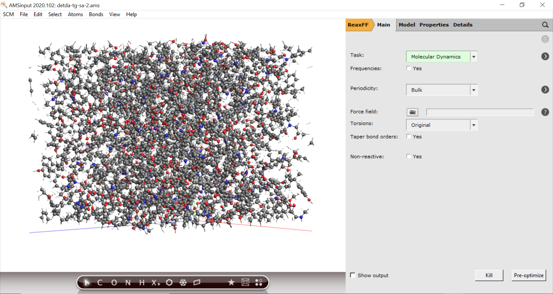
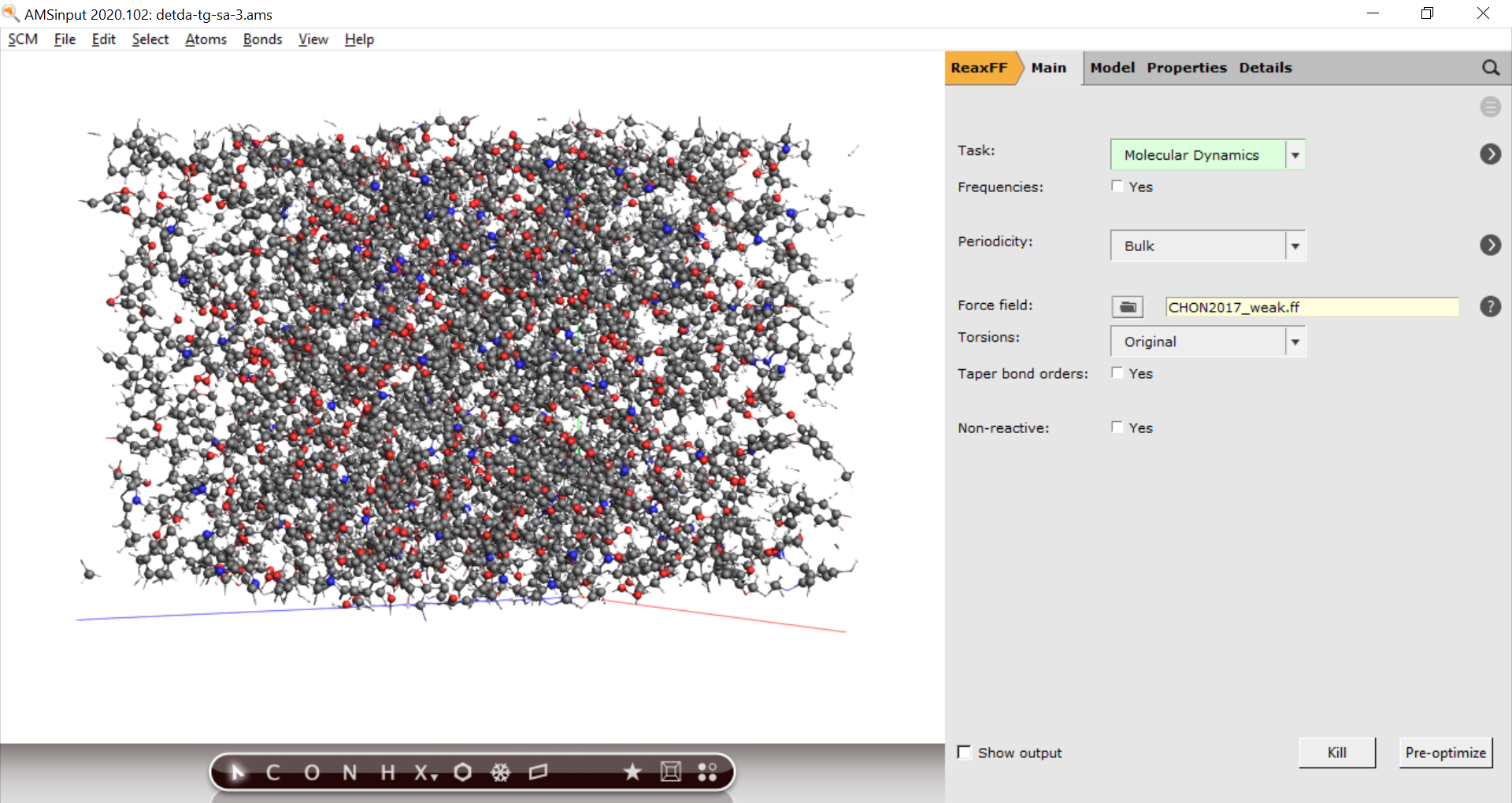
Start by choosing the MD settings:

1. In the main panel, select Task → Molecular Dynamics

2. Choose the force field CHON2017_weak.ff

3. Click on next to Task: Molecular Dynamics to go to the MD details

4. Set the Number of steps to 650000

5. Set the Sample frequency to 2000

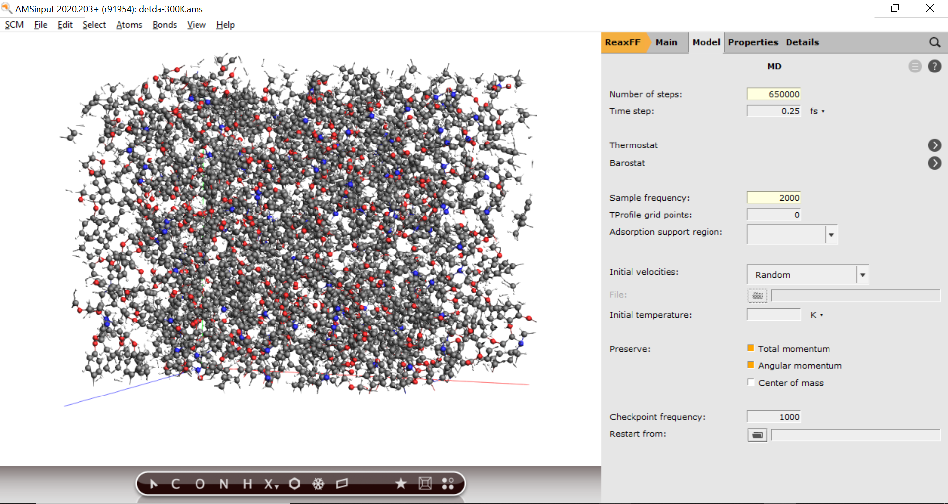
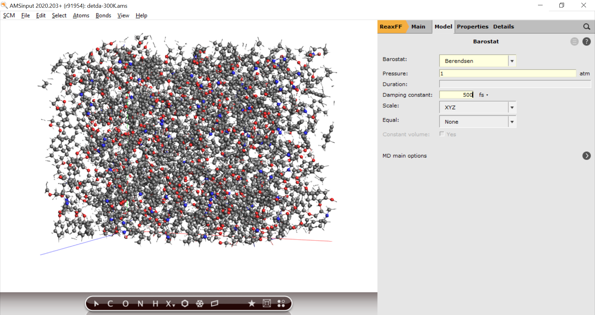
To allow the unit cell to shrink or expand we further add a barostat:

1. Click on next to Barostat

2. Select Berendsen from the Barostat dropdown menu.

3. Set the desired Pressure to 1.0 atm.

4. Set the Damping constant to 500 fs.

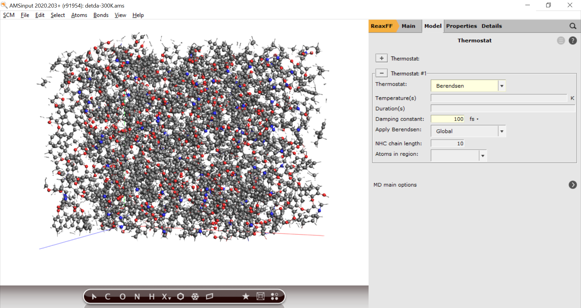
The annealing is defined in the thermostat panel

1. Click on next to MD Main options

2. Click on next to Thermostat

3. Select Thermostat → Berendsen

4. Set the damping constant to 100 fs

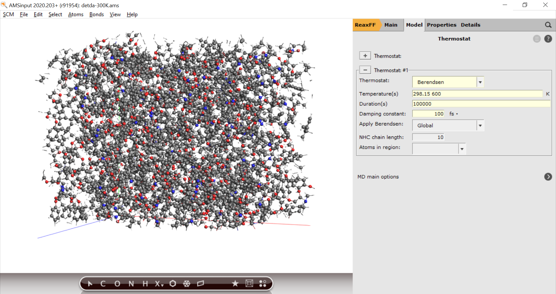
To increase the temperature from 298.15 to 600K over a duration of 100000 steps, followed by a cooling down back to 350K over a duration of 200000

5. Enter 298.15 600 350 into the Temperature(s) field

6. Enter 100000 200000 into the Duration(s) field

then to stepwise cool down to 300K again:

7. Add 350 340 340 330 330 320 320 310 310 300 300 to the Temperature(s) field

8. Add 50000 10000 50000 10000 50000 10000 50000 10000 50000 10000 50000 into the Duration(s) field

We are now ready to start the calculation

1. File → Save As… and give it an appropriate name (e.g. “CTE”)

2. File → Run

Extracting strain vs. temperature profiles

To extract the strain and temperatures from the trajectory for post-processing we make use of a Python script.

1. Download the script strain.py from here

2. Place it in the same folder as your CTE.ams inputfile

Next, you need to open the command line to execute the script with the AMS Python interpreter.

Tip

Windows and Mac users should open a pre-configured command-line from the GUI

In the command line, the script can be executed as follows

$AMSBIN/plams strain.py -v resultsdir=CTE.results -v startstep=300000

# T[K] a[Å]     b[Å]    c[Å]    V [Å**3]
350.4 85.121 70.228 90.103 538628.483
349.1 85.056 70.040 90.475 538988.118
347.8 85.309 69.796 90.124 536617.975
350.3 84.836 69.976 90.170 535290.469
350.2 84.862 70.100 90.187 536503.084
349.1 84.613 70.046 90.683 537466.316

but you can easily write them to file called strain.out instead:

$AMSBIN/plams strain.py -v resultsdir=CTE.results > strain.out

Calculation of the thermal expansion coefficient

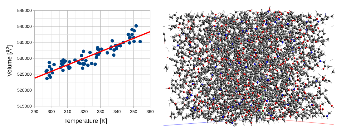
The strain can be plotted with any graph plotting software, e.g. gnuplot or any spreadsheet software. Import the results file into the software of choice and plot two column #5 (volume) against column #1 (temperature) and

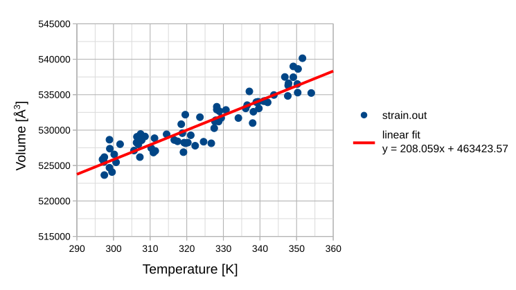
Perform a regression analysis and determine the slope. Calculate the thermal expansion coefficient (α₀) from the volume of the first data point (V₀) and the slope of the linear fit curve:

\[\alpha_V = \frac{1}{V_0} \frac{\partial V}{\partial T}_p = \frac{1}{538628.483} \cdot 208.059 = 38.6 \cdot 10^{-6} [1/C^{\circ}]\]

The simulated expansion coefficients is in the correct order of magnitude but underestimating the experimental expansion coefficient of 52.4 · 10^-6[1/°C]. This result is in line with the findings of the original publication Effect of chemical structure on thermo-mechanical properties of epoxy polymers: Comparison of accelerated ReaxFF simulations and experiments, Polymer 159, 354-368 (2018).