Glass transition temperatures of thermoset polymers

In this ReaxFF tutorial the calculation of glass transition temperatures, T_g, from the temperature dependence of the polymer’s density is explained.

The systems and workflows presented here are originally described in the publication Effect of chemical structure on thermo-mechanical properties of epoxy polymers: Comparison of accelerated ReaxFF simulations and experiments, Polymer 159, 354-368 (2018).

The tutorial consists of the following steps:

• Importing the polymer structure
• Simulated annealing
• Extraction of density vs. temperature profiles
• Calculation of the glass transition temperature

Note

The calculations are computationally demanding. For optimal performance, a parallel execution on a compute cluster is advised. This can best be done by using the remote job management of the GUI

Importing the polymer structure

The tutorial will use a cross-linked epoxy polymer generated with the bond boost method (see also bond boost tutorial ).

Begin by downloading the polymer and import into AMSinput:

Click here to download the .xyz file detda-epoxy.xyz

Import the coordinates in AMSinput:

File → Import Coordinates

Simulated annealing

In order to accurately simulate the temperature dependence of the density, we will have to make sure that the polymer structure is as homogeneous as possible. Large holes inside the polymer structure are an indicator for an inhomogeneous structure that will result in very noisy and hard to analyze results.

Simulated annealing is a simple optimization strategy intended to yield the global minimum energy structure on a complex and high dimensional potential energy surface. During the annealing the temperature during an MD simulation is gradually increased, hoping that the system can overcome more and more energy barriers and explore the energy landscape effectively. The heating phase is followed by a cool down period in which the system is cooled back down to the initial temperature. Often the resulting structure is significantly lower in energy than the starting structure, though there is no guarantee it is the optimal one.

Start by choosing the MD settings:

1. In the main panel, select Task → Molecular Dynamics

2. Choose the force field CHON2017_weak.ff

3. Click on next to Task: Molecular Dynamics to go to the MD details

4. Set the Number of steps to 970000

5. Set the Sample frequency to 5000

To allow the unit cell to shrink or expand we further add a barostat:

1. Click on next to Barostat

2. Select Berendsen from the Barostat dropdown menu.

3. Set the desired Pressure to 1.0 atm.

4. Set the Damping constant to 500 fs.

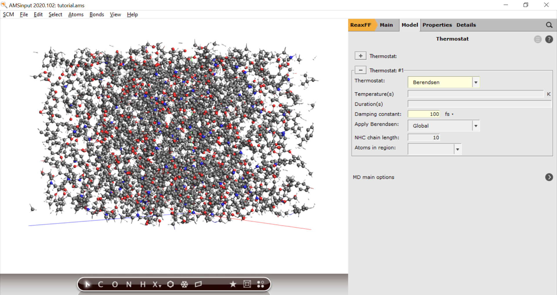
The simulated annealing is defined in the thermostat panel

1. Click on next to MD Main options

2. Click on next to Thermostat

3. Select Thermostat → Berendsen

4. Set the damping constant to 100 fs

Next, we define the desired temperature program. For the extraction of densities from the calculation we shall increase the temperature from 298.15 to 598.15 which is still low for a simulated annealing but sufficient for our purpose.

The temperature program we want to implement is simple:

• Heat up by 25 K over the course of 30000 steps
• Sample the density over a course of 10000 steps
• Repeat until reaching 598.15 K, then reverse to cool down to 298.15 K again

The individual steps of this program can be entered into the input fields Temperature(s) and Durations. In our case it’s easiest to copy and pastem them into the GUI.

1. Copy the individual temperatures from the following list

Temperatures::

298.15 298.15 323.15 323.15 348.15 348.15 373.15 373.15 398.15 398.15 423.15 423.15 448.15 448.15 473.15 473.15 498.15 498.15 523.15 523.15 548.15 548.15 573.15 573.15 598.15 598.15 573.15 573.15 548.15 548.15 523.15 523.15 498.15 498.15 473.15 473.15 448.15 448.15 423.15 423.15 398.15 398.15 373.15 373.15 348.15 348.15 323.15 323.15 298.15 298.15

2. Paste them into the Temperature(s) field

3. Copy the individual ranges from the following list

Durations::

10000 30000 10000 30000 10000 30000 10000 30000 10000 30000 10000 30000 10000 30000 10000 30000 10000 30000 10000 30000 10000 30000 10000 30000 10000 30000 10000 30000 10000 30000 10000 30000 10000 30000 10000 30000 10000 30000 10000 30000 10000 30000 10000 30000 10000 30000 10000 30000 10000

4. Paste them into the Duration(s) field

We are now ready to start the simulated annealing calculation

1. File → Save As… and give it an appropriate name (e.g. “SimulatedAnnealing”)

2. File → Run

Extraction of Density vs. Temperature profiles

To extract the densities and temperatures from the trajectory for post-processing we make use of a Python script.

1. Download the script densities.py from here

2. Place it in the same folder as your SimulatedAnnealing.ams inputfile

Next, you need to open the command line to execute the script with the AMS Python interpreter.

Tip

Windows and Mac users should open a pre-configured command-line from the GUI

In the command line, the script can be executed as follows

$AMSBIN/plams densities.py -v resultsdir=SimulatedAnnealing.results

Calculation of the glass transition temperature

The density profiles can be plotted with any graph plotting software, e.g. gnuplot or LibreOffice calc. Import the file into the plotting software of choice and plot the two columns against each other. The graph will fall into one of two categories:

If the final density of the initial structure and the equilibrated structure differ significantly and the experimental density (if available) is far off, then the density is not converged and another simulated annealing run should be carried out. If the final and initial density are close, then the simulation can be considered converged and one can proceed with the calculation of T_g.

To calculate T_g, carry out two linear fits through the data points as shown in the below figure. The intersection between these two lines marks the glass transition temperature.

The subsets of points for the linear fits should be chosen such that a maximum R₂value is obtained. If the R₂values are too low, i.e. the data is too noisy, or the curves don’t intersect, we advise to try one of the following troubleshoots:

• Run another simulated annealing simulation
• Extend the temperature range
• Reduce or increase the averaging parameter in the densities.py script