Realistic-temperature fuel pyrolysis with collective variable-driven hyperdynamics (CVHD)

Overview

This advanced tutorial demonstrates the use of a novel acceleration technique called collective variable-driven hyperdynamics (CVHD).

The tutorial is based on the results presented and discussed in the publication Kristof M. Bal and Erik C. Neyts, Direct observation of realistic-temperature fuel combustion mechanisms in atomistic simulations, Chem. Sci., 2016, 7, 5280

Note

This tutorial uses the fast empirical ReaxFF engine to run an example simulation in about an hour on common hardware. You can also select a different AMS engine such as DFTB or MOPAC in the first step, but then the simulation will likely take several days.

Background information

When dealing with acceleration techniques it can be helpful to revisit some of the fundamental problems and ideas associated with rare events. An outline of this information is given in this subsection. If you want to jump forward to the hands-on part of tutorial, click here.

Many interesting problems are driven by rare events, i.e. events that take place far outside the realm of accessible timescales in molecular dynamics simulations. These events can be chemical reactions (catalysis, industrial, enzymes) or physical processes (diffusion, phase transitions).

To illustrate the scaling problem we are dealing with, assume a hypothetical “wonder CPU” that can compute one MD time step (1fs) per clock cycle (1 ns). Even with this ideal machinery, simulating 1 s of dynamics will require 10 ⁶wall-s (12 days). Brute-force MD is not feasible and one needs to come up with a different strategy.

Two main approaches are commonly used

• Lowering the effective barrier - biased MD
• Cherry-pick interesting trajectories, e.g. parallel replica dynamics, transition path/interface sampling

The biased MD philosophy can be summed up into two steps: First, running the dynamics using a modified potential or equations of motion to accelerate, followed by an un-biasing in which the effect of the bias is removed from the results.

Free-energy methods (Potential of Mean Force) need to record the bias applied for the unbiasing step. For these methods, suitable collective variables (CVs) need to be defined to reduce dimensionality. In practice up to 2 (3) CVs are feasible (using methods like umbrella sampling, Metadynamics, adaptive biasing force, etc.). Alternatively, it’s also possible to sample along a one-dimensional reaction path using Nudged Elastic Band or the string method.

Either way, setting up a “good” CV is crucial for obtaining meaningful results. “Good” CVs should

• unambiguously define the state of the system (different states must not overlap)
• ensure that orthogonal processes average out
• be smooth and continuous

CVs in this sense are usually not trivial to construct and not suited for studying many independent simultaneous processes. To illustrate the idea, consider Metadynamics as a prominent example of a free energy sampling method. The bias - usually Gaussian - is periodically deposited at the current CV value ξ _i. It fills the energy values incrementally until there are no barriers left (diffusive regime).

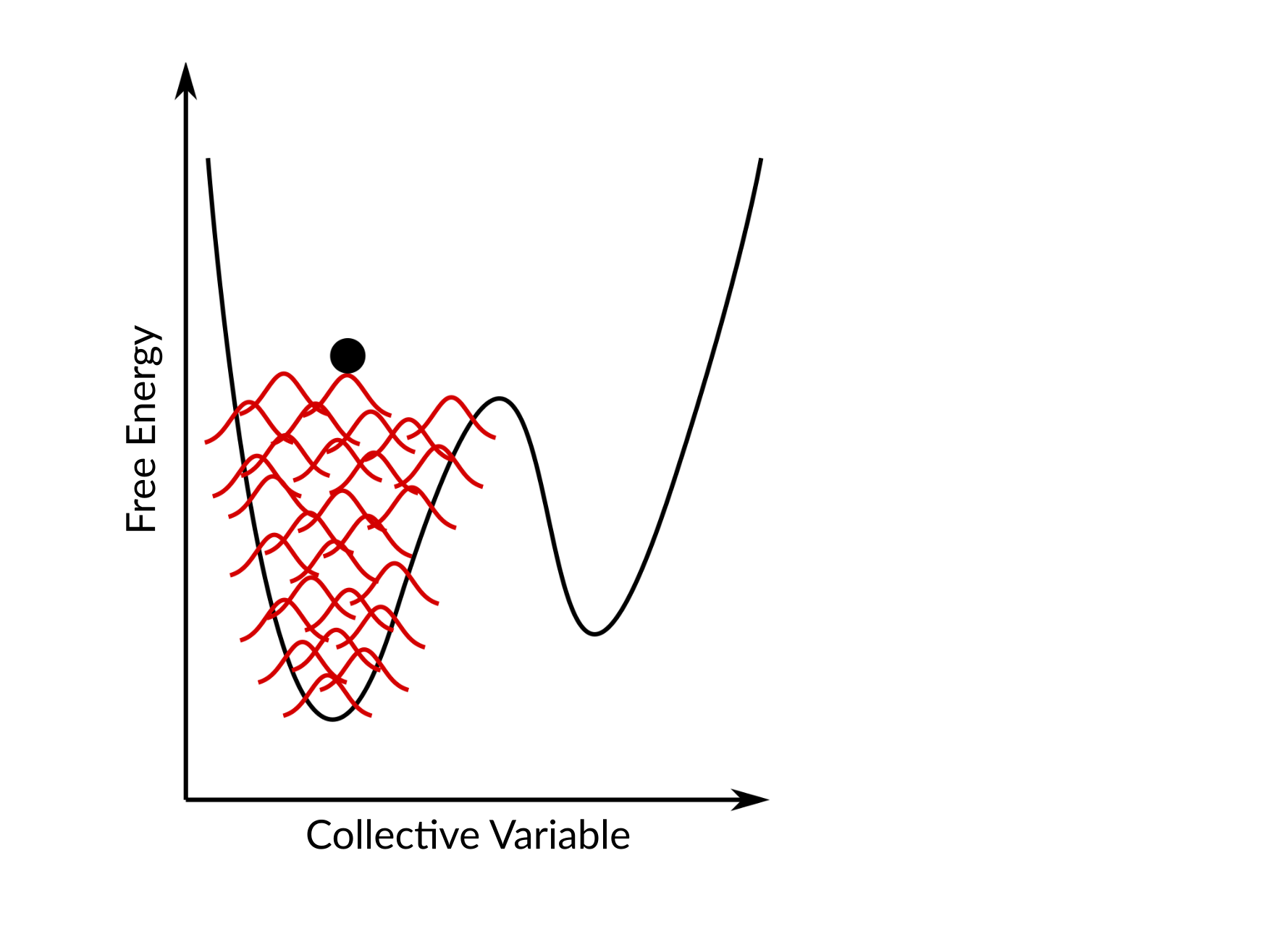
The free energy is then obtained as the negative of the converged V _bias

\[V_{bias}(\zeta) = \sum_{i}^{N_{biaspts}} g(\zeta-\zeta_i)\]

Alternatives to free energy sampling methods can be based on a biased sampling of trajectories, e.g. Transition Path Sampling or on on-the-fly unbiasing during the dynamics. The latter ansatz leads to Hyperdynamics. The free energy information is lost by the on-the-fly unbiasing but the time can be recovered from the simulation. When the simulation is run on a modified potential:

\[V'(x) = V(x) + V_{bias}(x)\]

the “hypertime clock” is advanced by

\[\Delta t_{hyper} = he^{V_{bias}(x)/(k_BT)}\]

In simple words, the Hypertime will tell you “How long would it take to get here in an unbiased simulation?”. It must be ensured that the transition state regions remain bias-free. Choosing a suitable bias V _biasfor Hyperdynamics is thus hard and error-prone.

A possible remedy is the use of self-learning bias, leading to CV-based Hyperdynamics (CVHD). In this approach V _biasis built on the fly using Metadynamics with a suitable CV η. As opposed to metadynamics, the bias is reset once a transition is detected. The CV now only needs to be valid for a single transition.

The global CV η is composed of primitive local CVs χ _iin such a way that it will be dominated by the highest χ _i.

\[\eta = \frac{1}{2}(1-cos(\pi\chi_{tot}^2))\]

\[\chi_{tot} = \bigg( \sum_{i}^{N}\chi_{i}^{p} \bigg) ^ {1/p}\]

At this moment in time only a bond-breaking local CV is implemented (see Bal and Neyts, J. Chem. Theory Comput. 2015 ):

\[\chi_{i} = \frac{r_i - r_{i}^{min}} {r_{i}^{max} - r_{i}^{min}}\]

\[0 \le \chi_i \le 1\]

The bias is applied to bonds approaching a transition - defined as the distance between r _i^max and r _i^min. The construction of these CVs means that when all bonds are near equilibrium, the global CV η is close to zero. As the bias builds up, it drives η to higher values, which in turn drives the currently most stretched bond in the system further towards dissociation. Once the CV η reaches 1 and stays at that value for a specified time, the algorithm assumes that a transition has occurred and resets the bias and the list of bonds.

Note

Only bonds that have bond order larger than the configured bond order cutoff at the beginning of the simulation are considered in the CV η. Additionally, some AMS engines have additional internal bond order cutoffs, thus imposing an effective minimum on the bond order cutoff. For example, the ReaxFF engine never returns any bonds with a bond order below 0.3.

The System

As a simple example, the low temperature pyrolysis of dodecane under realistic conditions (1000 K, 50 kg/m3) is simulated. This is a challenging reaction to simulate, because the pyrolysis products of alkanes depend on the temperature, resulting in the following trends:

• High T (> 2000K) - Ethylene is by far the dominant reaction product as entropically favored decomposition reactions become the dominant process.
• Lower T - Formation of larger 1-alkanes results in larger product molecules C3 and higher become much more dominant.

For this reason the dynamics of the low-T pyrolysis cannot just be simulated by increasing the simulation temperature. Also a brute force approach of the dynamics is not feasible given the rare-event nature of the bond breaking reactions as will become clear in this tutorial.

With respect to the paper, the following changes were made for the sake of computational efficiency

• The timestep was increased to 0.2 fs (→ lower accuracy)
• A smaller system of only 228 atoms is used

As a result there will not be enough data for proper statistics or rate constants. Still one can estimate the timescales of the different processes.

Preparation

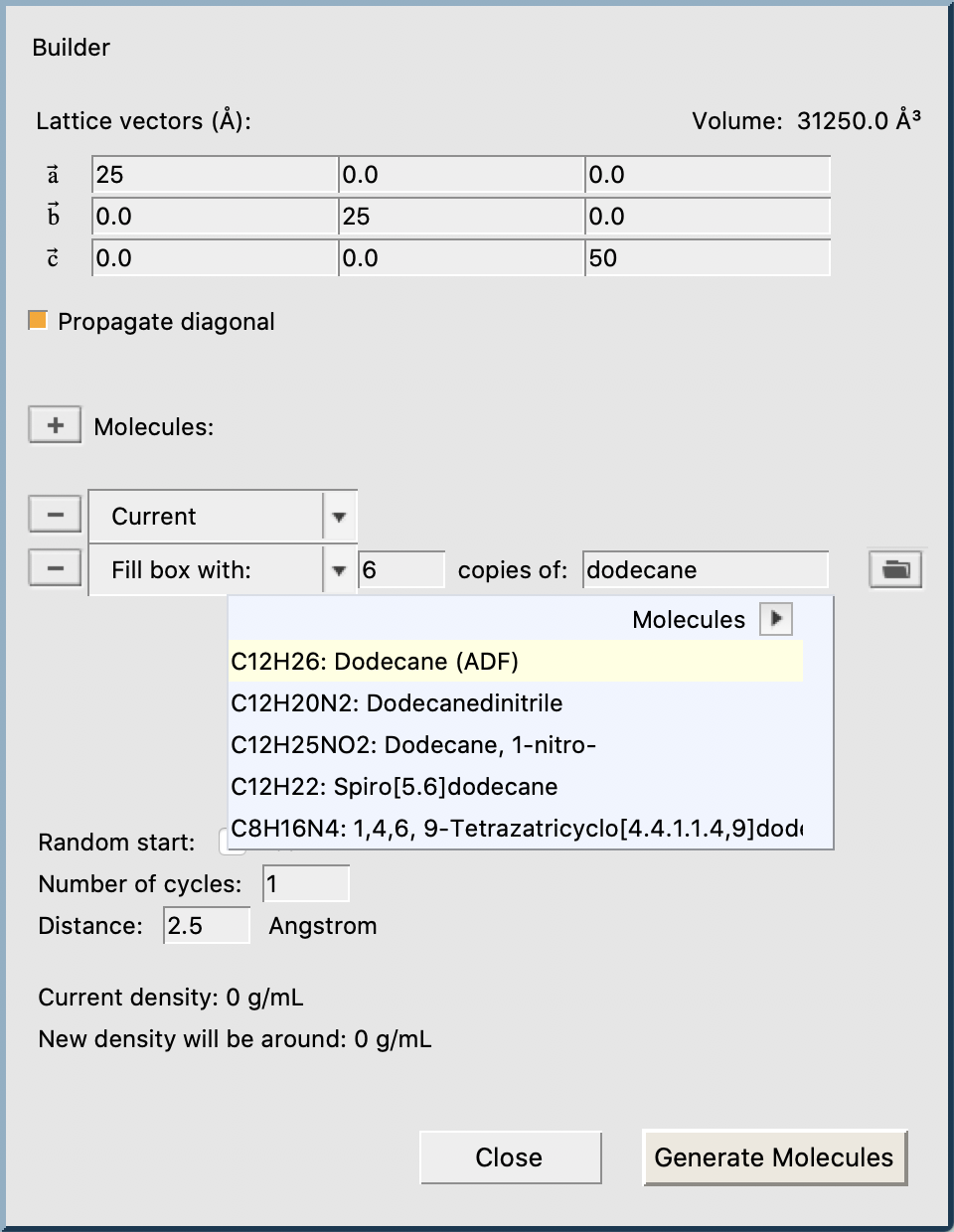
Begin by packing a periodic box with 6 dodecane molecules:

Switch to the ReaxFF module

Edit → Builder

Enter 25, 25 , 50 on the diagonal to create a 25x25x50 Å box

Enter dodecane into the text field and select Dodecane (ADF)

Enter 6 into the textfield Fill box with

Click Generate Molecules and Close

Use the following settings:

Select the CHO.ff force field

Make sure that Task is set to Molecular Dynamics and click the arrow to the right

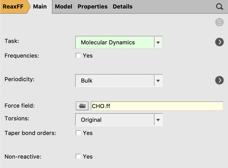
Enter a timestep of 0.2 fs

Set the number of steps to 2000000

Set the sampling frequency to 1000 steps

Set the checkpoint frequency to 100000 or more

Click the arrow to the right of “Thermostat”

Note

The absolute minimum of steps needed to see a reaction is one million steps (20-40 minutes depending on your hardware). However more steps are strongly recommended (at least 1.5-2 million)

Note

Because we’re using a small system with a fast engine like ReaxFF, it makes sense to adjust the frequency at which the MD simulation is checkpointed to enable restarting in case of a crash. By default, this is done every 1000 MD steps, meaning that a checkpoint would be written every few seconds. Here we have increased this period to reduce the checkpointing overhead.

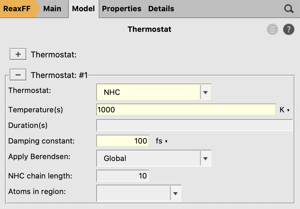
Click on the “+” button next to “Thermostat:”

Select the NHC thermostat

Set a temperature of 1000 K

Set the damping constant to 100 fs

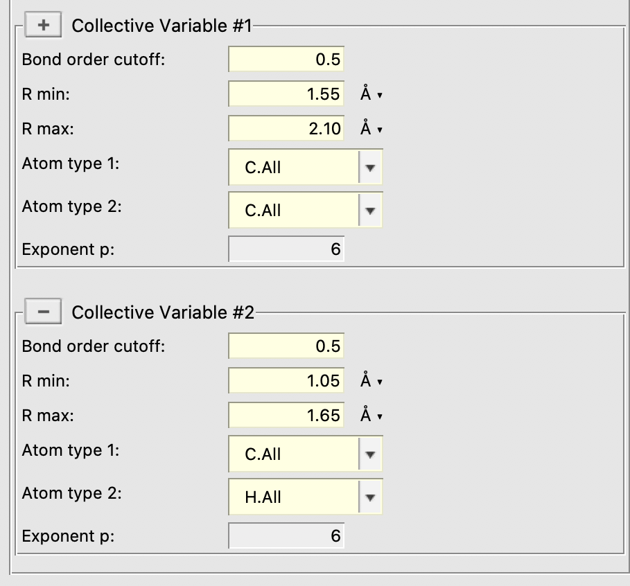
Finally, two local collective variables are setup

• C-C with Rmin = 1.55 Å and Rmax = 2.10 Å
• C-H with Rmin = 1.05 Å and Rmax = 1.65 Å

Note

The collective variables and their parameters are taken from the paper by Bal and Neyts, with the sole exception of the Rmax for C-C. This value was adjusted from the published 2.20 Å to give more reliable results with this small model system and limited simulation time. You can, of course, use the original published value instead or tune it yourself as discussed below.

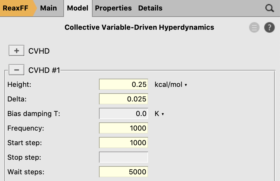
Go to Model → Collective Variable-Driven Hyperdynamics

Click the “+” button next to “CVHD”

Set the “Bias height” to 0.25 kcal/mol

Set bias Delta to 0.025

Enter 1000 as the deposition frequency

Enter 1000 as the Start step

Set Wait steps to 5000 steps

Use the “+” button next to “Collective Variable #1” to bring up two CV blocks

Enter the CV settings listed above

Save and Run

CVHD events in the output

While the calculation is running, you can inspect the output:

Select Output from the SCM menu

The HyperTime is the “true” timescale after unbiasing, i.e. how long a process would take without CVHD. After the first 1000 unbiased steps, bias starts building up and the simulation gradually accelerates:

• after 1 ps (5000 simulation steps), a speedup of 23% is already reached
• after 20 ps (100 000 simulation steps), 2.4 ns have been sampled
• after 40 ps (200 000 simulation steps), 71 ns have been sampled

At a later stage of the simulation the system will approach a transition which manifests as a slowdown in the hypertime evolution as there will be no bias in the transition state region. In the current example, a molecule dissociates around simulation step 920 000.

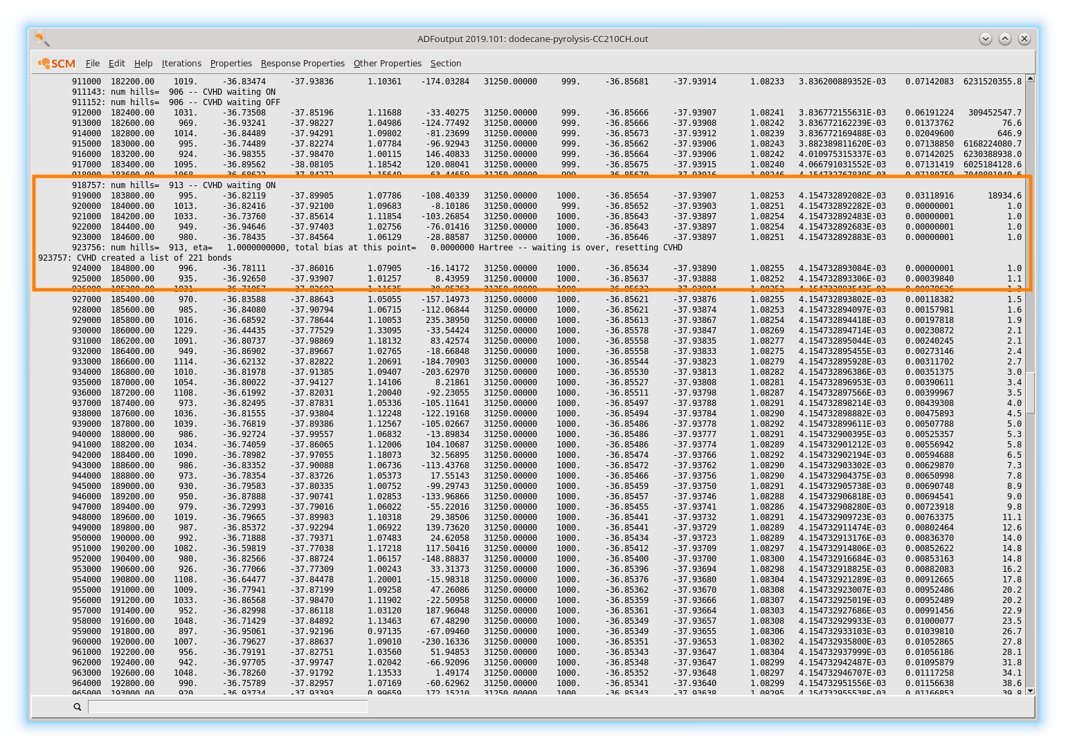
At this moment the algorithm will wait for 5000 steps (as requested in the settings) to see if the system recrosses back into the original state. No recrossing occurs, so CVHD declares that an event (reaction) just took place and removes all bias. A new set of bonds participating in the collective variable is then detected around step 924 000 and new bias starts building up.

Analyzing the System Composition

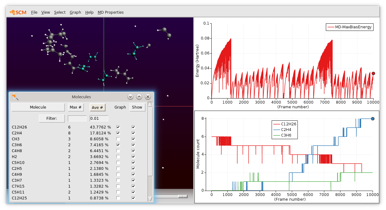
You can use AMSmovie to watch the simulation as it runs and to inspect the reactions more closely. For example, you can plot Max Bias Energy to see how the CVHD bias gradually builds up and how it is reset when an event occurs.

Open AMSmovie (select Movie from the SCM menu)

Remove the default energy plot using Graph → Delete Graph

MD Properties → Max Bias Energy

Add a second graph panel using Graph → Add Graph

MD Properties → Molecules

Check Graph to plot the number of particular molecules/fragments

Tip

Click on a curve to highlight corresponding molecules.

An example showing the consumption of dodecane (red) and the production of ethylene (blue) and propene (green) from a longer (10 million steps) CVHD trajectory looks as follows

Monitoring the bias deposition

Note

This analysis step uses the command line. On Windows and Mac the command line can be opened from within any GUI module via Help → Command-line (Windows) or Help → Terminal (Mac). See also the Getting Started page of the scripting docs.

It is possible to monitor the deposition of the bias using a small command line script called cvhd-hills.py. To plot where the biasing hills are deposited

Open a command line window

Type $AMSBIN/amspython $AMSHOME/scripting/standalone/reaxff-ams/cvhd-hills.py path/to/jobname.results and hit ENTER

Tip

To change the name of the output file, supply the new name as an additional argument.

This will generate an output file called cvhd-hills.csv that will be opened in AMSgraphs automatically.

Change the default plotting mode of AMSgraphs to Data Points:

Plot → Options → Curves

uncheck Curve and check Data Points

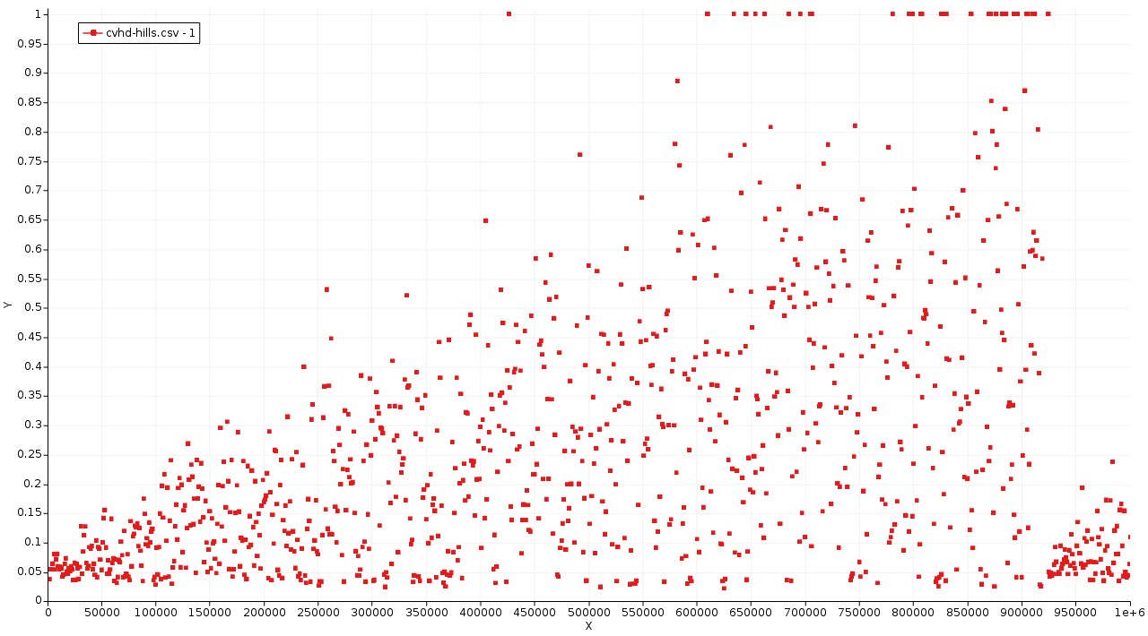
Now you should see a plot similar to the one below.

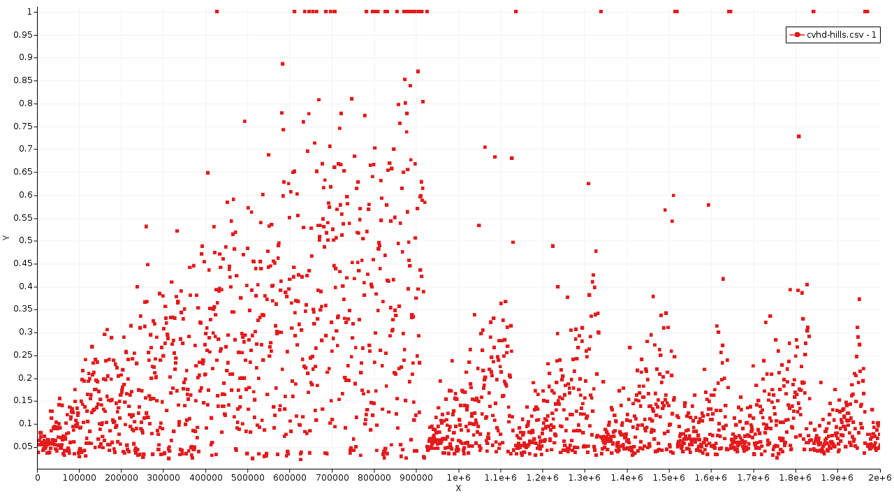
In this graph the MD step is on the x-axis and the CVHD global collective variable η on the y-axis. Each point represents a single Gaussian bias hill. As an exception, the points at η = 1 only denote that the system visited the transition region. The CVHD method never deposits bias above η = 0.9.

Let’s take a closer look at the first CVHD event.

Initially, the system stays around η = 0 (all bonds relaxed). With the build up of the bias, η is gradually pushed to higher and higher values (bonds are stretched more and more). On some occasions from on iteration 400 000, η reaches 1.0 but returns back to lower values. This means that during the specified wait time no transition occurred. Finally, around step 900 000 η stays at 1.0 long enough to indicate that a bond has dissociated.

Improving the CV using the Bias Deposition Plot

The above bias deposition plot can be used to improve the collective variable using the following diagnostics:

Initial η not close to zero

Rmin is set too low. CVHD “thinks” the equilibrium structure is already partly dissociated

η doesn’t freely explore higher values (stays close to zero for a long time)

Rmin is set too high

Too many recrossings: η keeps hitting 1.0 but no true reaction occurs

Rmax is set too low, not close enough to a transition.

System jumps from low η directly to 1.0, triggering a reaction

Rmax is set too high, past the transition state.

It’s often useful to tune each local CV (bond type) separately before combining them in a single simulation. The global CV contains a weighted sum of local CVs resulting in an optimal Rmin that is system-size-dependent. Typically, large systems need a somewhat higher Rmin.

Analyzing Event Timescales

Note

This analysis step uses the command line. On Windows and Mac the command line can be opened from within any GUI module via Help → Command-line (Windows) or Help → Terminal (Mac). See also the Getting Started page of the scripting docs.

The hypertime associated with each CVHD event can be plotted with the help of the script cvhd-hypertime.py:

Run $AMSBIN/amspython $AMSHOME/scripting/standalone/reaxff-ams/cvhd-hypertime.py path/to/jobname.results

Tip

Per default the output file is called cvhd-hypertime.csv. To change the name of the output file, supply the new name as an additional argument.

Change the y-axis in AMSgraphs to a logarithmic scale for best results:

Plot → Options → Left Y axis

Make sure the Minimum value is set to a positive number, e.g. 1e-12.

Check Logscale

Plot → Options → Curves

uncheck Curve and check Data Points

Now you should see a plot similar to the one below.

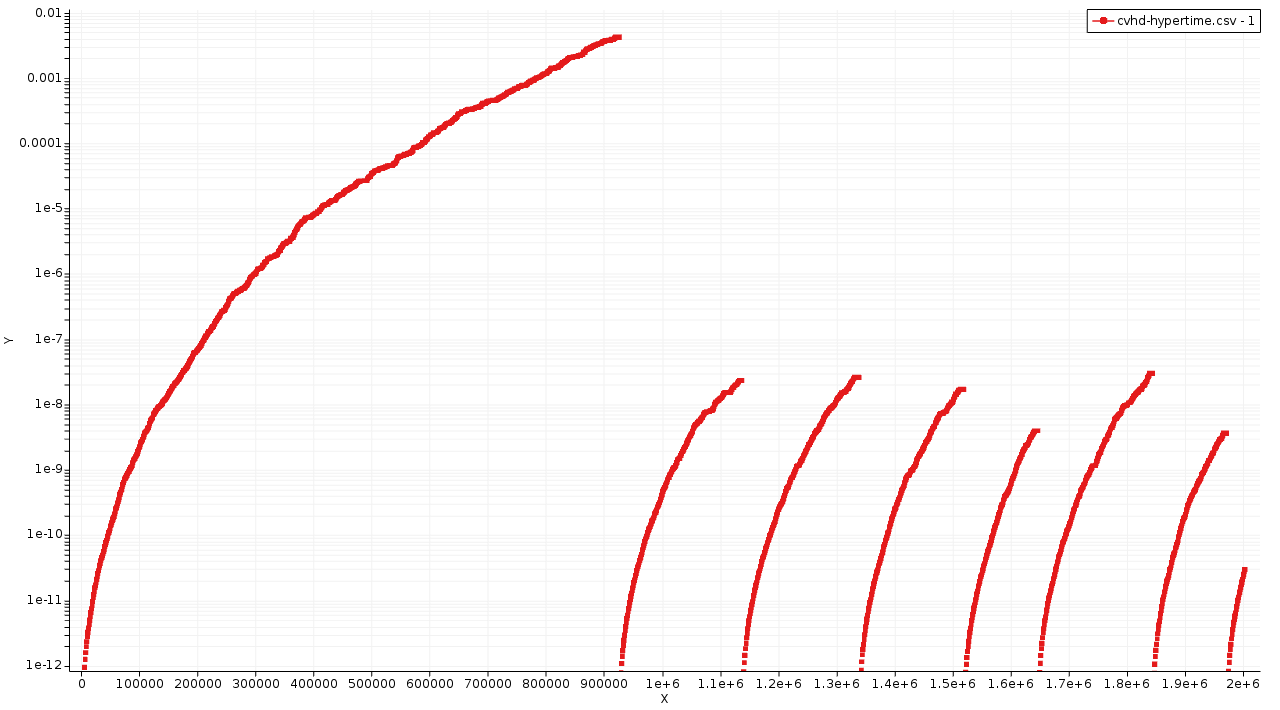
The x-axis shows the MD step and the y-axis the hypertime in seconds since the previous event. Each curve shows the gradual acceleration of time as the bias evolves until an event (bond dissociation) is detected. The curves show classes of processes corresponding to different timescales are visible

• The Initiation step (dodecane chain splitting) at a millisecond timescale.
• Propagation steps occur at a ns-μs timescales

The curves should be (mostly) smooth. Jagged or staircase-like curves indicate issues with the CVHD setup (Rmin/Rmax, deposition rate, etc…).

Discussion

This tutorial is using a small example system as well as a minimal amount of steps for the sake of computational efficiency. As a direct consequence

• we can’t expect any reasonable statistics or rate constants
• most elementary reactions are observed only once, some are completely missed
• only a rough order-of-magnitude estimate on timescales can be made
• multiple trajectories yield largely different results

To overcome these limitations, a bigger system and longer simulation times are required.

The chosen timestep of 0.2 fs is possibly to inaccurate during the transitions and the results should be verified using a shorter timestep (0.1 fs). Finally, the Rmin/Rmax parameters for the C-H bonds could probably benefit from further tuning with the help of the bias deposition plots.

Summary

The collective variable driven hyperdanymics ansatz implemented in AMS2019:

…is suitable for accelerating bond dissociation

Any process that starts with bond dissociation can be accelerated.

…has a relatively low setup effort

Only Rmin/Rmax distances are needed for each bond which can be estimated and tuned in a few short testing runs. The hill height and deposition rate may need to be adjusted depending on the expected barrier height.

…works best for moderately-sized systems

CVs comprising many thousands of bonds trigger events too often which limits bias buildup and acceleration. Only the number of biased bonds matter as opposed to the overall system size, and those can be limited using suitable regions. See the CVHD manual for more information.