QTAIM (Bader), (localized) orbitals and conceptual DFT

Step 1: QTAIM (Bader) analysis of Caffeine

Start ADFinput

Next we need a reasonable guess for the structure of Caffeine. The quickest way to do this is to search for it in the database of molecules included with the ADF-GUI, and optimize it:

Press cmd-F or ctrl-F to activate the search box

Type ‘caffeine’ in the search box

Move your mouse pointer on top of the ‘Thein’ search result

As you can see, there are several matches. If you position your mouse over the results (without clicking) a balloon will appear showing the details of that match. For this tutorial we use the second match “Thein”, from the NCI database. Thein is one of the common names for caffeine (and as you can see there are may alternative names).

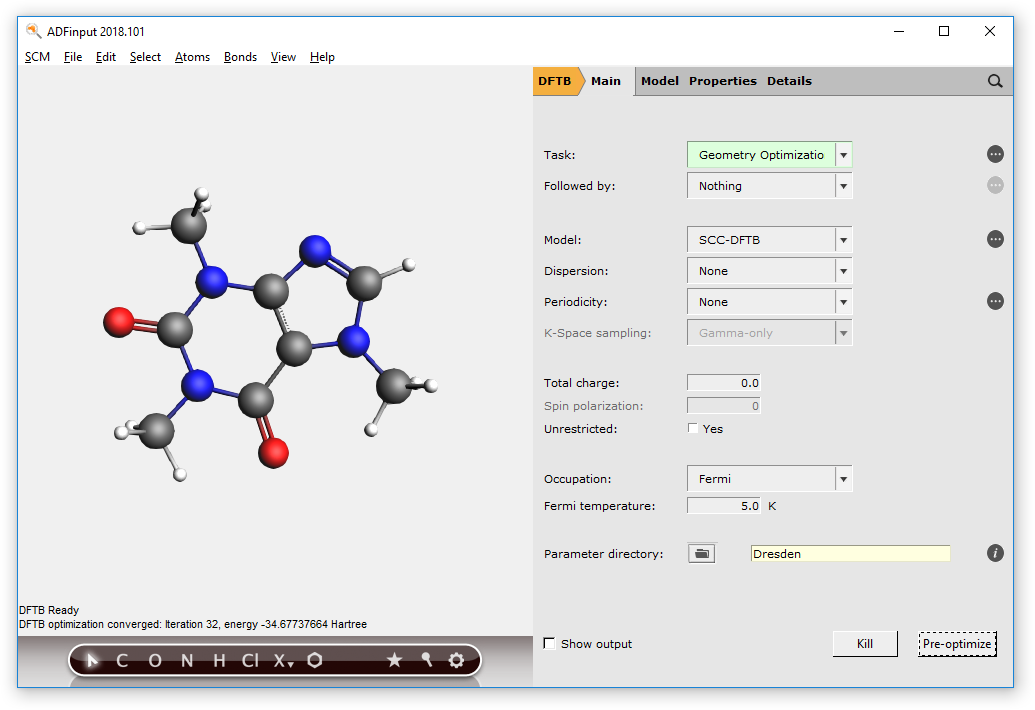
Click on the ‘Thein’ search result

Click somewhere in empty space in the molecule drawing area to deselect the atoms

Switch to DFTB mode (panel bar ADF → DFTB)

Select the “Dresden” parameter set (normally you would want to use better parameters like the included 3OB set)

Note that only those parameter sets known to be able to handle your system will be shown in the menu.

If you move your mouse over the parameter field, the information balloon will also show references applicable to the selected set of DFTB parameters. More detailed information and references will be displayed if you click on the button next to the parameter input field.

Click the ‘Pre-optimize’ button

If the message says ‘NOT converged’, press ‘Pre-optimize’ again.

The DFTB program should have created something similar to this structure:

Next we will calculate the AIM critical points and paths for the current structure.

Switch to ADF mode (panel bar DFTB → ADF)

Now we want to activate the Bader AIM analysis to find the critical points and bond paths. To find where this option is located, search for it:

Activate the search box (cmd/ctrl-F)

Type ‘criti’ in the search box

Click on the first hit ‘Other: Etot, Bader, Charge, Transport, ...’

ADFinput will switch to the panel that displays the option you are looking for (to calculate the AIM critical points and paths). The matching input options will be marked with blue italic text. Note that we first had to activate the ADF mode, the input option search will restrict the search to panels that belong to the current method (ADF, BAND, DFTB, ...)

Check the box to calculate Bader (AIM ) Critical points, bond paths and atomic properties

Check the box to calculate AIM atomic energies

Check the box to save the Bader basins

Run this setup: File → Run

A dialog will pop up in which you must specify a filename to use for your job, for example caffeine:

Enter ‘caffeine’ as a Filename, press the Save button

After hitting the save button the calculation will start. You will get two extra windows: first a window for ADFjobs that allows you to manage your jobs and keep track of their state (for example, queued or running). You will also get a window showing the ADF log file. This shows you what is going on in the current calculation.

Depending on your computer, the calculation should be ready after a few minutes at most:

Now use ADFview to visualize the results:

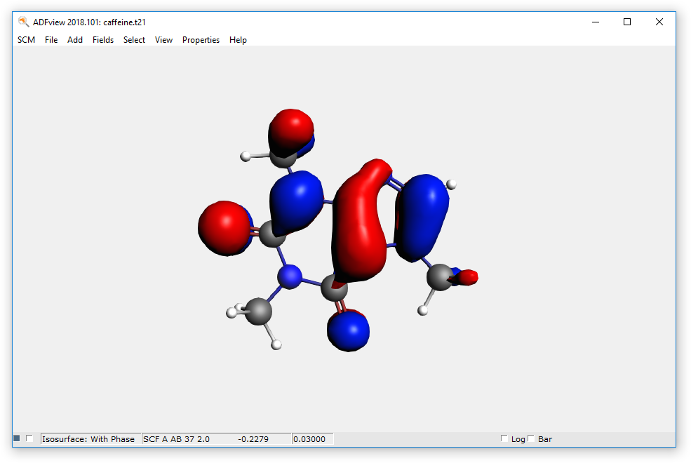
Start ADFview SCM → View

Show the HOMO Properties → HOMO

Hide the HOMO by unchecking the check box at the lower left corner of the ADFview window

Add → Isosurface: Colored

In the first field selector (to the right of the ‘Isosurface: Colored’ text at the bottom), select Density → SCF

In the second field selector (to the right of the ‘0.03’ text in the same line), select Potential → Coulomb Potential SCF

Hide the surface with the potential energy: uncheck the check box at the lower left corner of the window

Properties → AIM (Bader)

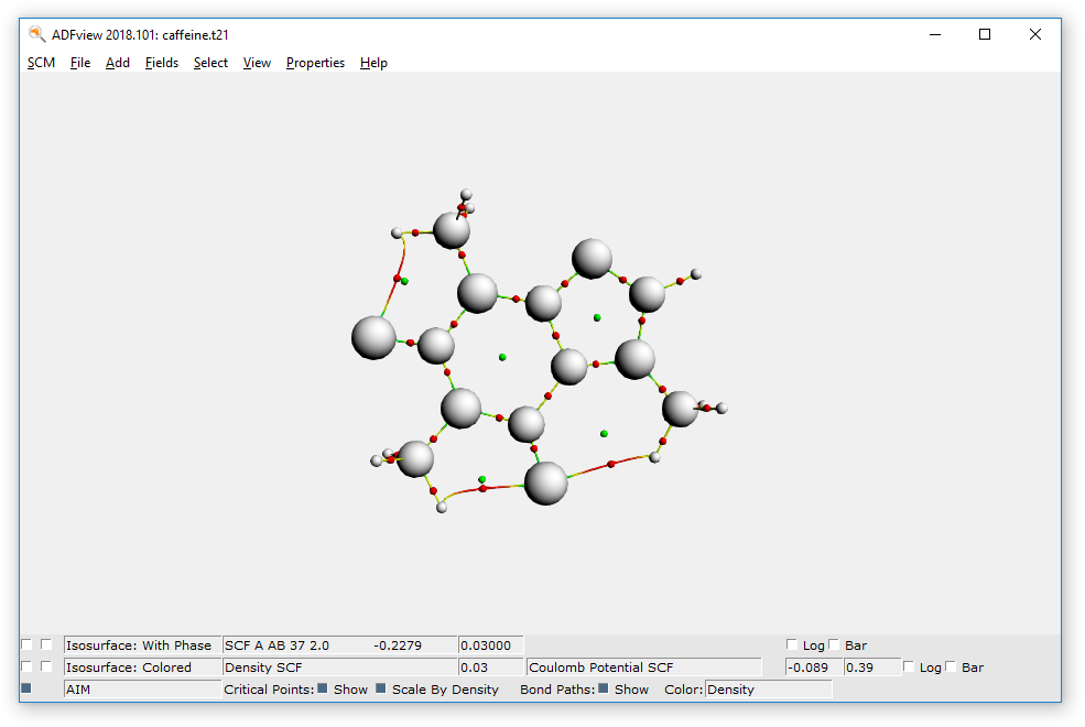
The critical points and bond paths are shown (the molecule balls and sticks representation is hidden). The different types of critical points (atom CP, bond CP, ring CP and cage CP) are indicated by different colors. The bond paths are colored by density, by default.

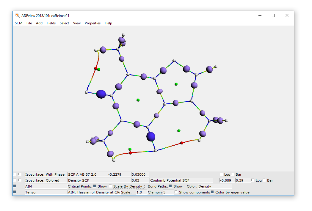
You can also visualize the Hessian of the Density in the critical points:

Properties → AIM: Hessian of Density at CPs

To get a rough display of the Bader basins, use the Bader sampling option:

Properties → Bader Sampling

Zoom in

The different colored points show the different basins.

ADFview has many options to visualize the results, the options just used are mainly to show off some features. Play around with the different options, for example try out what the check boxes do on the left side. Or try other fields, or colored cut planes, or ...

This finishes the Caffeine Bader (AIM) tutorial, close all its windows:

SCM → Quit

Step 2: Benzene Bader charge analysis and NBOs

Start ADFinput

Make a benzene molecule (for example by searching for it with cmd/ctrl-F)

Set up a Single Point calculation without frozen core (Frozen Core → None)

Panel bar Properties → Other: Etot, Bader, Charge Transport, ...

Check the ‘Atomic energies’ option

Panel bar Properties → Localized Orbitals, NBO

Check the ‘Perform NBO analysis’ option

Request Boys-Foster localized orbitals

Run this setup (File → Run)

When the calculation is done (it should run very fast), we use ADFview to examine the Bader charges and compare them with Mulliken charges:

Open the results with ADFview

Show the Bader atomic charges (Properties → Atom Info → Bader Charge → Show)

Color the atoms by Bader charges (Properties → Color Atoms By → Bader Charge)

Show the Mulliken charges (Properties → Atom Info → Mulliken Charge → Show)

Next we inspect the NBOs and Boys-Foster localized orbitals. To remove the charge display we close and open ADFview, but you could also have used the View menu to remove them by hand:

Close ADFview

Open the results again with ADFview

Add an isosurface with phase

Use the field menu in the new control line,

and observe the labels present with the NBOs and NLMOs

Open a NBO similar to BD Cn - Hn

Improve the grid by using Fields → Grid → Fine

Obviously, you can also visualize the NLMOs or the Boys-Foster localized orbitals (which are just called Localized Orbitals in the fields menu.

Step 3: Rationalizing a typical SN2 reaction using condensed Conceptual DFT descriptors

The chemical reactivity of reactants or key intermediates can be analyzed using condensed (over QTAIM basins) Conceptual DFT descriptors such as Fukui functions or Dual Descriptor. We strongly suggest the use of the Dual Descriptor, which gives at one glance a more complete description of reactivity behaviors. All the following calculations are based on frontier molecular orbitals (FMOs) using Koopmans approximation, which presents advantages (fast calculations) and drawbacks (in particular if FMOs are degenerated or quasi-degenerated).

An alternative way, based on finite difference linear (FDL) approximation, is available in ADF: Fukui Functions and Dual Descriptor. The FDL approximation offers a more rigorous approach, but it requires three calculations (systems with N electrons (reference), N+δ electrons and N-δ electrons (0<δ<=1)) and shows other drawbacks. For instance, adding one electron to the reference system may lead to unconverged SCF procedure, or the corresponding spin states might be unobvious. Besides, some ambiguity remains about which atomic basins (relaxed or unrelaxed) should be used when adding or removing electrons.

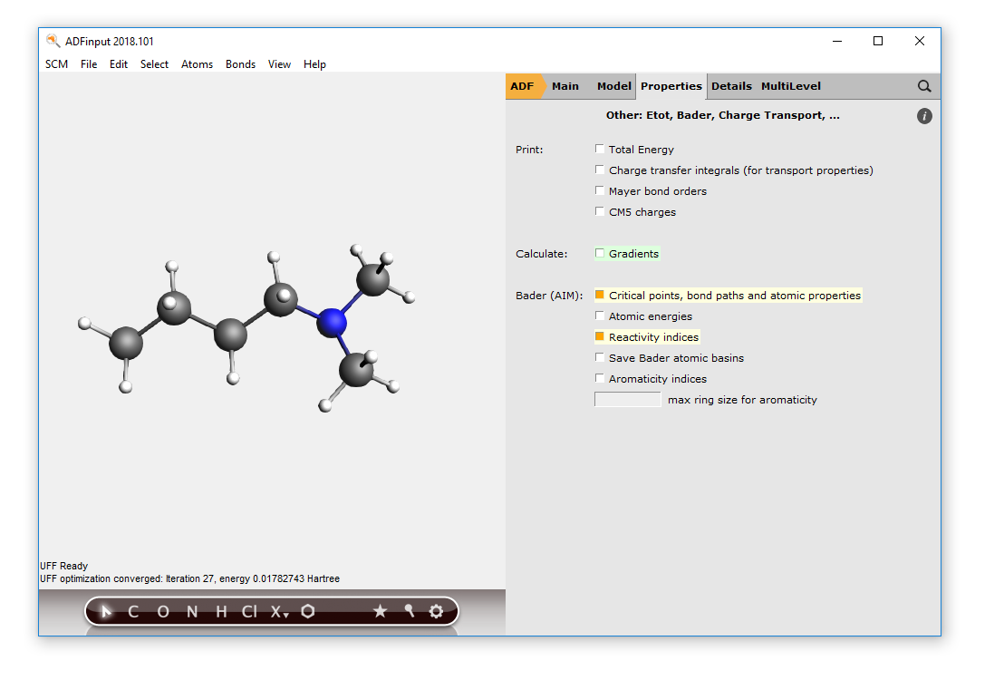
Start ADFinput

Draw the N,N-dimethylbutylamine molecule (nucleophile)

Pre-optimize the structure

Select the Geometry Optimization task

Panel bar Properties → Other: Etot, Bader, Charge Transport, ...

Check the ‘Bader (AIM) Critical points, bond paths and atomic properties’ option

Check the ‘Reactivity indices’ option

Run this setup: File → Run, use ‘nucleophile’ as file name for your job

Wait until it is ready, click then No when asked to update the coordinates in ADFinput

At the end of the optimization process, all the QTAIM properties will be calculated.

Start ADFview: SCM → View

Show the condensed (over QTAIM atomic basins) ‘Fukui Fminus function’ indices that characterize the nucleophilicity of atomic sites:

Properties → Atom Info → Fukui Fminus → Show

Properties → Color Atoms By → Fukui Fminus

Properties → Atom Info → Name → Show

On this picture, we clearly see that the nitrogen site is the most nucleophilic one. To obtain a more complete picture at one glance, we can visualize the condensed values of the dual descriptor (DD) that corresponds, using the Koopmans’ theorem, to the difference between FMOs electron densities.

To this end, first hide the previous values and display the condensed DD values:

Properties → Atom Info → Fukui Fminus → Hide

Properties → Atom Info → Koopmans DD → Show

Properties → Color Atoms By → Koopmans DD

Positive indices correspond to atomic sites where electrophilicity is predominant, while negative indices correspond to atomic sites where nucleophilicity is predominant (again, the nitrogen atom is highly nucleophilic).

In a new input window, now make the benzyl chloride (electrophile):

SCM → New input

Make benzyl chloride by copying the following coordinates:

C      -0.70294970       0.03823073       0.00000000
C      -0.02771734      -1.20050280       0.00000000
C       1.37040750      -1.24326069       0.00000000
C       2.10941268      -0.05859271      -0.00000000
C       1.45241936       1.17312771      -0.00000000
C       0.05527963       1.22223527      -0.00000000
C      -2.21056076       0.15917615      -0.00000000
Cl     -2.96962094       0.22007043       1.61845248
H      -0.56397603      -2.13845972       0.00000000
H       1.88164983      -2.19732981       0.00000000
H       3.19110656      -0.09523365      -0.00000000
H       2.02573037       2.09116490      -0.00000000
H      -0.43823632       2.18658642      -0.00000000
H      -2.49816320       1.08415158      -0.54318756
H      -2.64194499      -0.70811986      -0.54318753

Pre-optimize the structure

Select the Geometry Optimization task

Panel bar Properties → Other: Etot, Bader, Charge Transport, ...

Check the ‘Bader (AIM) Critical points, bond paths and atomic properties’ option

Check the ‘Reactivity indices’ option

Run this setup: File → Run, use ‘‘electrophile’’ as file name for your job

Wait until it is ready, click then No when asked to update the coordinates in ADFinput

At the end of the optimization process, all the QTAIM properties will be calculated.

Start ADFview: SCM → View

Show the condensed (over QTAIM atomic basins) ‘Fukui Fplus function’ indices that characterize the electrophilicity of atomic sites:

Properties → Atom Info → Fukui Fplus → Show

Properties → Color Atoms By → Fukui Fplus

Properties → Atom Info → Name → Show

On this picture, two carbon sites (C(4) and C(7)) have similar Fplus indices. Moreover, chlorine has a strong electrophilic character due to the existence of a sigma hole in the outer part of its valence shell along the C-Cl bond. Therefore, it is difficult to unambiguously determine the reactivity of this molecule by the sole QTAIM condensed Fplus values. In that case, the dual descriptor is quite useful, providing a balanced picture, since it allows evaluating the predominant reactivity behavior at each atomic site.

To this end, first hide the previous values and display the condensed DD values:

Properties → Atom Info → Fukui Fplus → Hide

Properties → Atom Info → Koopmans DD → Show

Properties → Color Atoms By → Koopmans DD

As already mentioned, positive indices correspond to atomic sites where electrophilicity is predominant, while negative indices correspond to atomic sites where nucleophilicity is predominant.

On this picture, we clearly see, as expected from chemical intuition, that C(7) is highly electrophilic (compared to the other carbon atoms). This site will thus undergo a nucleophilic attack during the SN2 reaction with the N,N-dimethylbutylamine molecule, leading to the formation of a quaternary ammonium salt.

Besides, we can also observe that the chlorine atom is predominantly a nucleophilic site (due to its lone pairs) despite the presence of an electrophilic sigma hole.

SCM→ Quit All