H-NMR spectrum with spin-spin coupling
Learn how to use the GUI to setup the calculation of NMR chemical shifts and nuclear spin-spin coupling constants (NSSCCs). Use the ADFspectra module to inspect the results and compare the simulated and experimental NMR spectra directly.
See also
- Don’t miss this must-read FAQ entry on NMR settings based on the work done by the group of Jochen Autschbach
- The NMR part of the ADF manual contains a neat summary of the science behind spin-spin coupling calculations as well as some additional advice.
- The advanced tutorial on relativistic NMR calculations .
Step 1: Start ADFinput
The tutorial is best run in a separate folder labelled Tutorials
- Start ADFjobsClick on the folder icon labelled
TutorialsStart ADFinput using the SCM menu
Step 2: Create the molecule
You can download a pre-optimized ethyl acetate structure from here:
- Click
hereto download the .xyz file Ethyl_acetate.xyzImport the coordinates in ADFinput:File → Import Coordinates
The above structure was optimized with the following settings:
- Hybrid:PBE0
- Basis: TZP
- Frozen core: None
- Numerical Quality: Good
In case you want to run the geometry optimization yourself, take a look at the GUI tutorial on geometry optimizations.
Step 3: Setting up the NMR calculation
Select the following settings from within ADFinput
- XC functional: GGA → OPBEBasis set: J → TZ2P-JFrozen core: NoneNumerical quality: Good

Note
The basis sets in J, including TZ2P-J, have been especially designed for ESR hyperfine and NMR spin-spin coupling calculations.
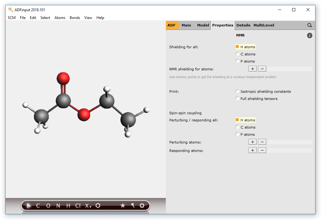
Next, instruct the program to calculate the shieldings for all hydrogen atoms.
- Click Properties menuSelect NMRClick checkbox H atoms next to shielding for allClick checkbox H atoms next to Perturbing / responding all
Note
In some cases, e.g. when dealing with alcohol groups, you might want to exclude atoms from the list of perturbing and responding atoms. To do so, just select the atoms you want to calculate the splittings for, and use the + button to add to the list of perturbing and responding atoms manually.
You have now finished the setup of the calculation and are ready to run it. It should take around 10 minutes to finish, but that may vary depending on your hardware.
- Select File → RunClick OK to save over the previous versionClick Yes when ADFjobs warns that results are already presentWait for the calculation to finish
Step 4: Results of your calculations
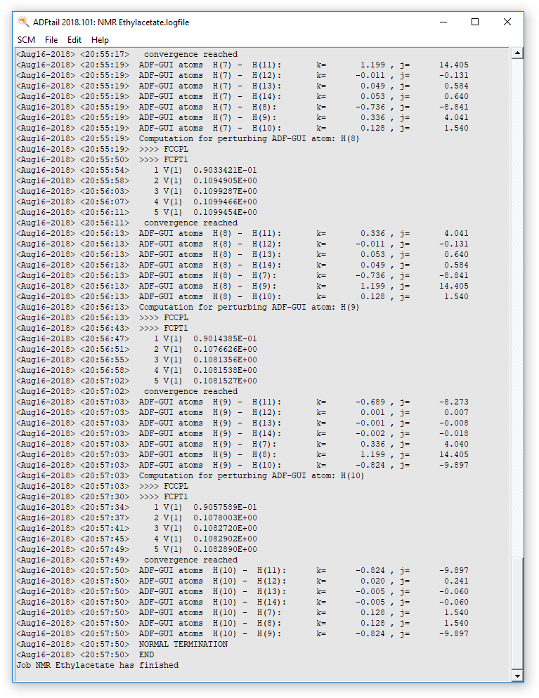
Logfile: ADFtail
You can follow the progress of the calculation with ADFtail. The chemical shifts will be calculated first, followed by the couplings constants for the perturbing and responding atoms.
When the calculation is finished the end of your logfile will look something like this:
View the 1 H-NMR spectrum
Use ADFspectra to visualize the calculated spectrum
- Select SCM → SpectraIn ADFSpectra, set the “Width” to 0.01

By default only the chemical shifts are visualized using plain singlets. To switch on the visualization of couplings:
- Click on the coupling checkbox
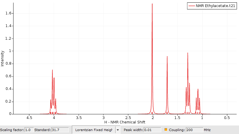
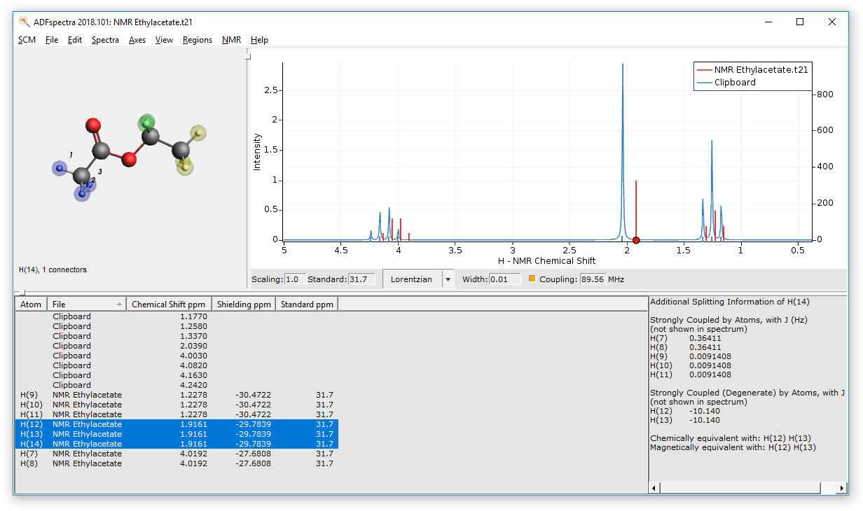
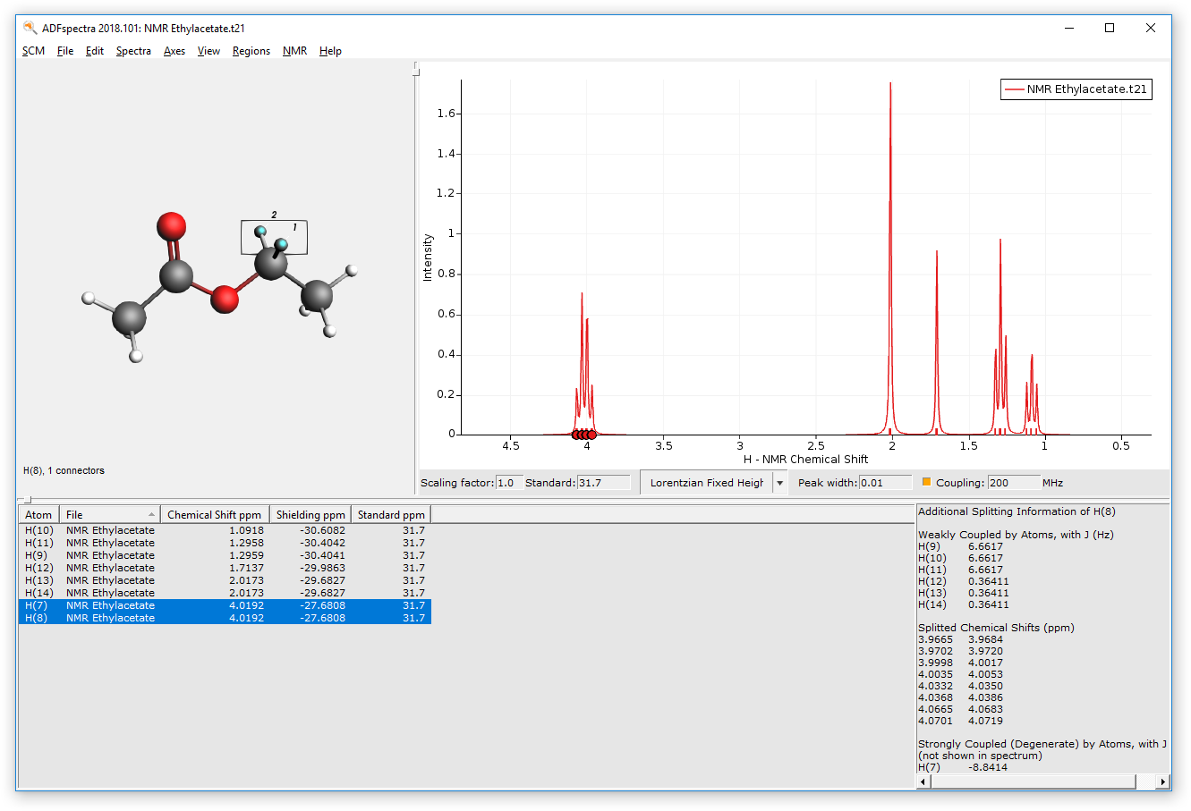
This switches on the spin-spin coupling (default machine frequency at 200 Mhz). An additional section in the table will appear which displays additional information for any selected atom or peak in the spectrum. For example:
- Click on the quartet in the spectrum

Average chemical shifts and couplings for equivalent atoms
As you may have noticed, there are a lot of splittings in the simulated spectrum. This is because all the chemical shifts and coupling constants are calculated at fixed geometry, which means that there is no rotation which would create magnetically equivalent groups.
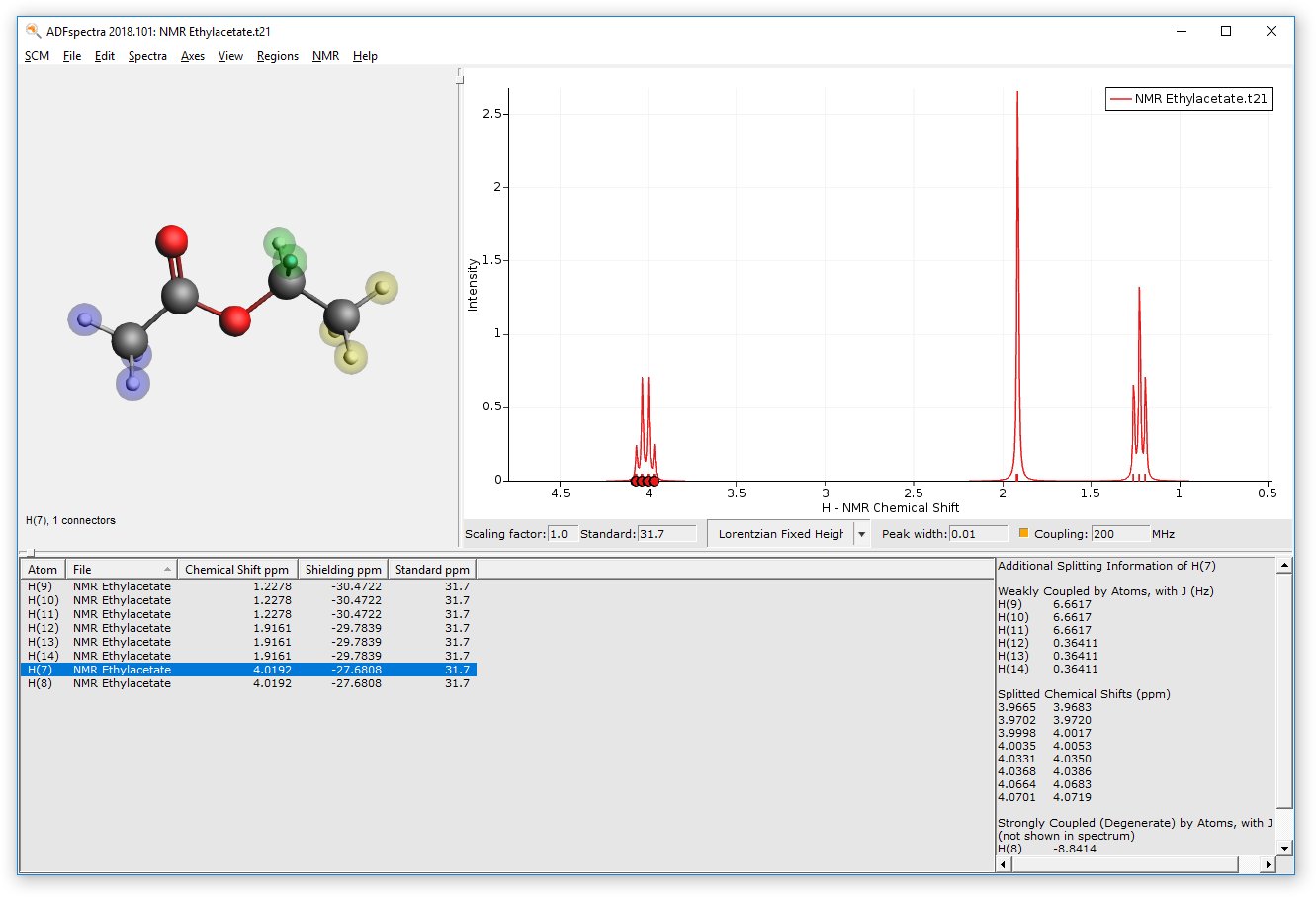
You can resolve this issue by either flagging chemically equivalent atoms manually or have ADFspectra guess them for you. To manually supply the information:
Select groups of chemically equivalent atoms and
- Hold down the SHIFT key on your keyboardUse the left key of the mouse to select several atomsPress CTRL+G or go to Regions → New Region From Selected Atoms
The atoms should now be surrounded by a colored sphere. Continue with all remaining atoms. Your spectrum should look as follows now:
To have ADFspectra guess chemically equivalent regions for you, go to
- Click on NMR menuClick on Chemical Equivalent Regions
Tip
In the NMR menu you can adjust the thresholds that are used by the algorithm to identify equivalent regions.
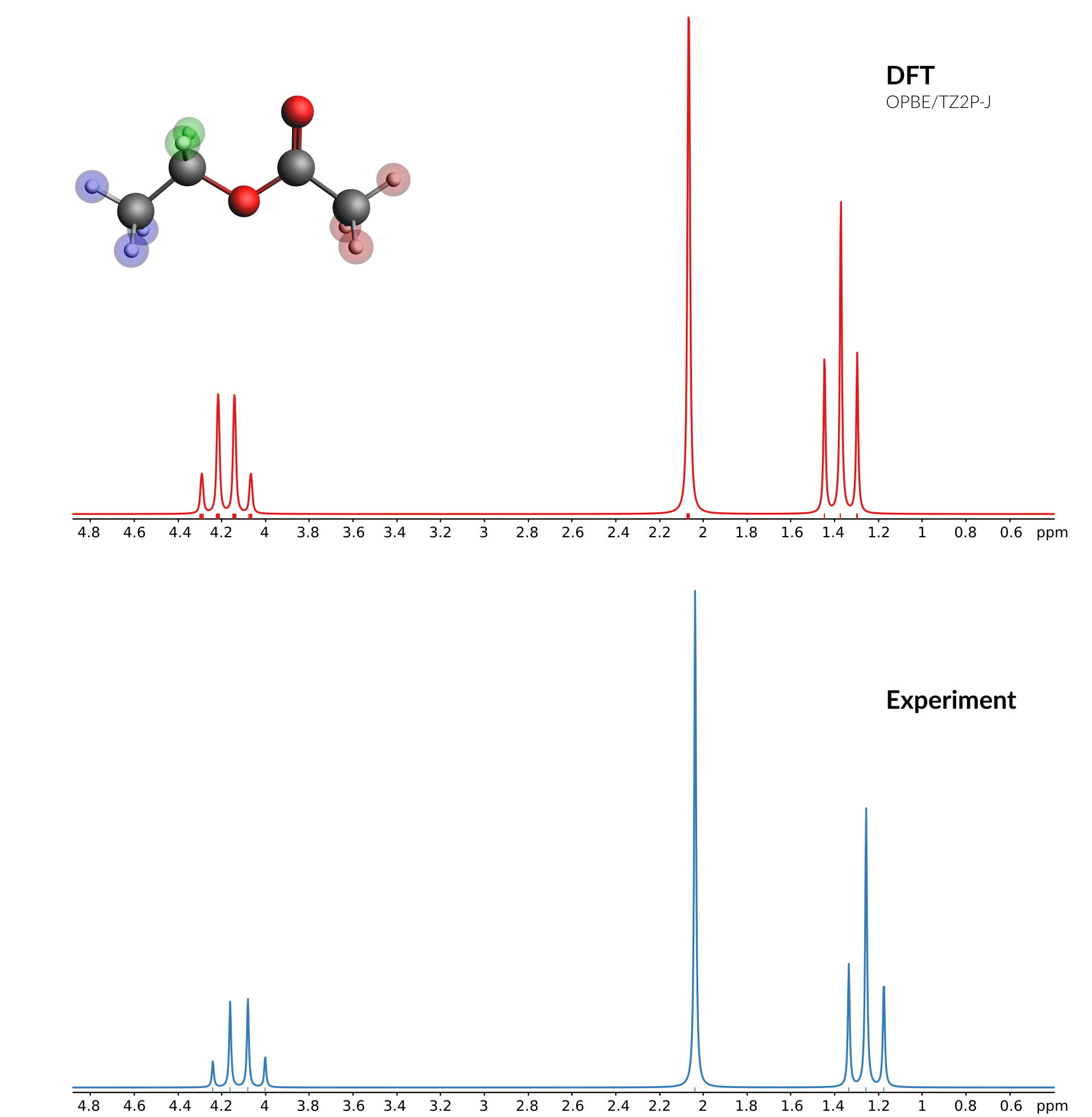
Comparison of calculated and experimental spectrum
A good source for experimental spectra is the SDBS database: http://sdbs.db.aist.go.jp/sdbs/cgi-bin/direct_frame_top.cgi
We will get the 1 H-NMR spectrum from that database and compare it with the calculated results. You can use data from any source you like, as long as data is avaiable as peaks (positions and intensties) or as a full spectrum (all X values with corresponding Y values).
As this part of the tutorial depends on external data, you may need to adjust details as needed.
- Use a browser (do NOT quit ADFspectra) to go to the SDBS database at http://sdbs.db.aist.go.jp/sdbs/cgi-bin/direct_frame_top.cgiSearch for ethyl acetate (CAS = 141-78-6)Select HNMR
You should see the 1H NMR spectrum, three groups of peaks, with assignment. Next we will copy the peak data to the clipboard:
- Click on the ‘Peak data’ buttonSelect the peak data (three columns, all lines with peaks)Copy
Now we switch back to ADFspectra where we can paste the contents from the clipboard directly:
- Activate the ADFspectra window showing the calculated ethanol spectrumEdit → Paste
ADFspectra will ask which columns to use for X and Y, and offer to rescale the data:
- Enter
2to use the second column as X values (that column contains the chemical shift in ppm) and click OKEnter3to use the third columns as Y vales and click OK
You now should see both the experimental and the calculated spectrum in one graph. The experimental spectrum (at least the one used to create this tutorial) was measured at 89.56 MHz. So adjust the frequency (default at 200 MHz) of the calculated spectrum:
- Change the frequency (next to the Coupling check box) from 200 MHz to
89.56MHz
This should give you something like this:

Sometimes it makes sense to change one of the spectra to a stick spectrum, showing only sticks for the calculated positions and heights, not applying the broadening. As an example lets do that here for the calculated peak positions:
- Double click below the X-axes to show the Graph options dialogClick on the Curves tabSelect the NMR curve (not the Clipboard one) in the menu on the leftFor this curve, on the right side: Show the Sticks, and do NOT show the Curve itselfClick OK
Now you should get the experimental spectrum as a broadened curve, with sticks for the calculated positions: