Discharge voltage profiles during lithiation using grand canonical monte carlo
Overview
This advanced ReaxFF tutorial will teach you how to calculate the discharge voltage profile of a LiS battery.
Contents:
- Importing a CIF file from an external database and equilibrating the structure
- Calculating the chemical potential for Li
- Setting up a grand canonical monte carlo (GCMC) simulation w. ReaxFF
- Results: How to calculate the discharge voltage profiles.
If you are not familiar with using the GUI yet, you might take a look at the ReaxFF GUI tutorials before continuing.
The System
This tutorial uses a small alpha-sulfur system consisting of 128 atoms. Both the system and the workflow presented here are originally described in the publication “ReaxFF molecular dynamics simulations on lithiated sulfur cathode materials” by M.M.Islam et al.
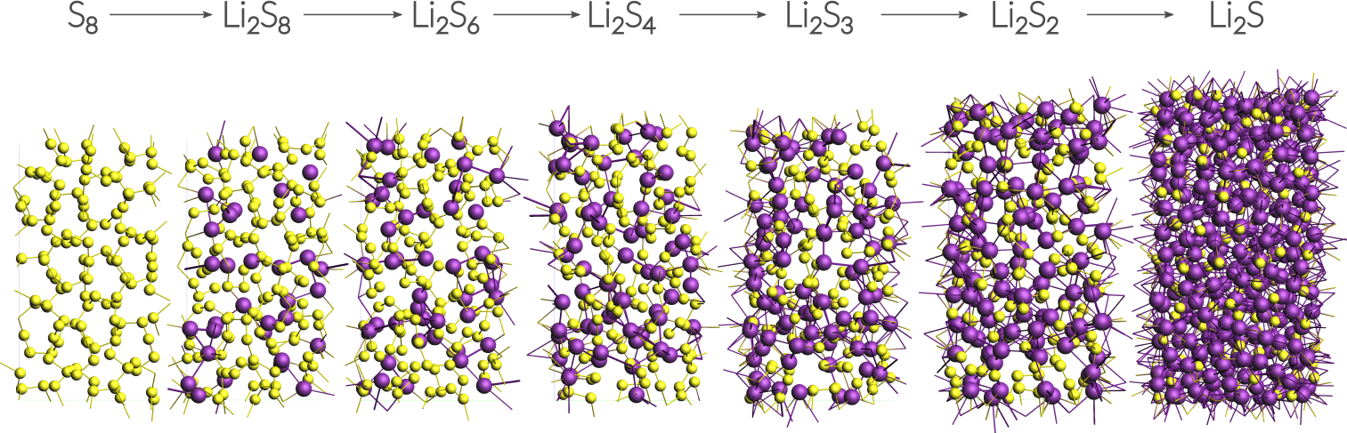
The discharge process is simulated using ReaxFF in a grand canonical monte carlo scheme. Volume changes upon lithiation are accounted for by using an NSPT-μLischeme. The discharge voltage can be calculated from the total energies of the lithiated compounds.
Importing the Sulfur(α) crystal structure
The crystal structure can be directly imported from a CIF file. There are several resources for crystollgraphic data available online and you can choose according to your liking. Here we use a structure of S8 alpha sulfur from the American Mineralogist Crystal Structure Database.
The downloaded CIF can directly be imported into ADFinput:
- File → Import CoordinatesEdit → Crystal → Map atoms to (0..1)View → Periodic → Show lattice vectors
The latter two steps map the coordinates into the ReaxFF unit cell and display the lattice vectors.
Before adding any Li-ions to the system, we need to relax the structure using a geometry and cell optimization, i.e. including the optimization of lattice vectors.
Tip
Often we find that running a couple of hundred steps NPT dynamics at low temperature and 0.0 pressure using a small timestep is sufficient as a relaxation or at least speed up a subsequent geometry optimization significantly.
With the current system we can run a geometry and cell optimization directly:
- Select the LiS.ff force fieldSelect Task → Geometry OptimizationSwitch to Details → Geometry OptimizationSelect Conjugate GradientSet the max. steps to
5000Select Cell Optimization → Full Cell
Save and run the calculation to yield a total energy of
Calculating the chemical potential for Li
Following the literature approach, we fix the external chemical potential of Li at the total energy of a single lithium atom in body-centered cubic lithium. The structure of bcc Lithium can be created easily via the crystal builder from within ADFinput:
- Edit → Crystal → Cubic → bccSelect Li from the Presets and click OKEdit → Crystal → Generate SupercellEnter
8,8,8on the diagonal to create an 8x8x8 supercell (512 atoms)Edit → Crystal → Map atoms to (0..1)
Optimize the resulting structure and lattice using the same settings as with the sulfur.
After the optimization has finished successful, the chemical potential is calculated as the total energy / number of atoms.
Note
The exact value depends to some minor extent on the chosen force field and for consistency one should always use the value predicted by the force field at use.
Throughout this recipe the LiS.ff is used and the chemical potential of Li will be fixed at
Setting up the GCMC calculation
GCMC calculations are quite sensitive to the chosen settings. The main reason being the interplay of comparing small energy differences in the GCMC acceptance criteria and the optimization procedure carried out after each MC-trial move.
Note
Its advised to try different optimizer settings (max. steps, convergence criteria, etc...). The GCMC settings are documented online (here).
The ADF development version (>= r62841) comes GUI support for GCMC calculations. We will be using the GUI in this tutorial but the same calculation can be run from the commandline as well.
Our previously optimized S8 structure will serve as the system:
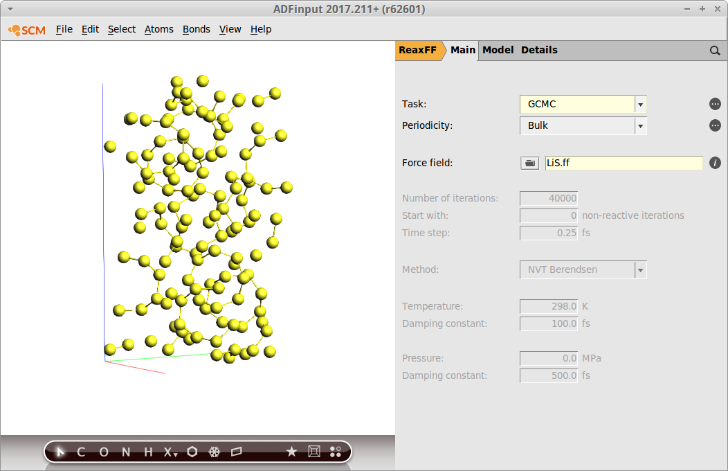
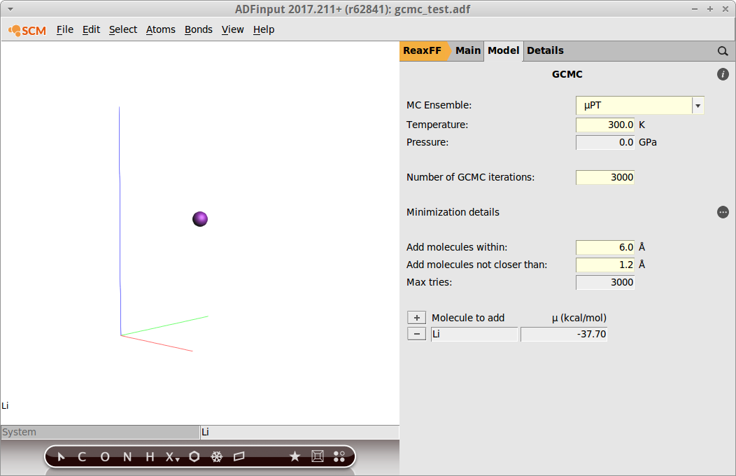
- Task → GCMCSwitch to the GCMC panel: Model → GCMCSelect MC ensemble → μPT
This will be enough steps to converge the current system. However, this value is not known beforehand and one might want to choose a larger number of iterations for larger systems.
- Set Temperature to
300Add molecules between1.2and6.0Å
These fields correspond to the Rmax and Rmin values in the GCMC input. You can try different values here.
As a complete empirical rule of thumb: setting Rmin to roughly ½ of the shortest expected bond and Rmax approx. half of the shortest lattice vector seems a good starting point.
- Max. tries →
3000
The number of attempted tries must be sufficiently large. If this is not the case, the calculation will abort with an error message stating that number of max tries was exceeded.
- Molecule to addPress the button labelled +Enter
Lias the name
The name is generic, you will still need to draw a Lithium atom into the window labelled “Li” in the molecule view to the left. After placing the Li-atom, select it place it in the middle of the unit cell as follows
- Edit → Crystal → Set(0.5,0.5,0.5)
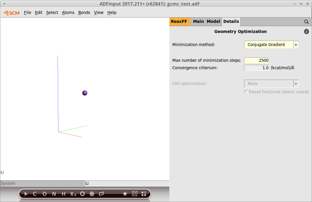
The optimizer settings can be found by clicking on the button labelled ”...” next to Minimization details. Remember that the optimizer settings are most crucial for the GCMC algorithm:
- Select Minimization method → Conjugate GradientSet Max. number of steps to
2500
Save your changes and run the calculation. The initial stages of the calcaulation are reached quite fast and the progress can be followed in ADFmovie. However, it will typically take a bit less than one day until convergence.
GCMC Troubleshoot
No MC-moves are accpted:
- Check if you set the correct chemical potential (remember to use the one calculated with your force field!)
- Tighten the convergence criteria for the optimization
- Change
RmaxandRminsettings - Try to optimize the system (here: the sulfur structure) with tighter optimization settings
- Try a different force field
The calculation takes a lot of time:
- Loosen the convergence criteria, e.g. less steps and a lower convergence criterium
- The obvious: Try a smaller system.
Results
The discharge voltage profiles can be calculated as a function of Li intercalation content from
where \(G\) denotes the Gibbs free energy and \(x\) the concentration of Li-ions. The enthalpic (PT) and entropic (TS) contributions can be neglected and thus the Gibbs free energy replaced by the ground state energy.
In this case and many other cases of non-standard trajectory analysis, writing a short Python script using the PLAMS library is the most efficient way to obtain results. Remember there is no need to take any further action than writing the script: Both Python and PLAMS are shipped with every copy of ADF/ReaxFF.
The script called LiVoltageProfile.py is available here and can be run as follows from the command line:
$ADFBIN/startpython LiVoltageProfile.py gcmc_test.rxkf
assuming that your trajectory was called gcmc_test.rxkf and that you used the same system and force field as explained in this recipe.
The results are written to a file called voltage_profile.out:

Lit.:
[1] M. M. Islam, A. Ostadhossein, O. Borodin, A. Todd Yeates, W. W. Tipton, R. G. Hennig, N. Kumar and A. C. T. van Duin ReaxFF molecular dynamics simulations on lithiated sulfur cathode materials, Phys. Chem. Chem. Phys. 17, 3383-3393 (2015).